A spiral capacitor
A spiral capacitor is a two-pin capacitor whose electrodes are two interleaved spirals. Every turn of one arm has the other arm on both sides, so a small cut-out in the ground plane holds a long, thin gap and a lot of capacitance. Use one when you want a series capacitor between a feedline and a resonator that is larger than an interdigital capacitor of the same footprint. This page builds it step by step: the geometry, the two pins, a LOM model, and a chip that uses it.
The finished files are examples/custom_component/spiral_capacitor.py and the notebook
examples/custom_component/custom_passives.ipynb. It assumes you have read
Components.
What you build
Part |
Choice |
|---|---|
Class |
|
Category |
|
Pins |
|
Parameters |
|
LOM |
one |
Step 1: the geometry of the arms
Both arms are Archimedean spirals, r = r_in + pitch * t / 2π. Arm A starts at angle 0, arm B at 180 degrees. The
radial distance between two turns of one arm is pitch = 2 * (arm_width + arm_gap), so the other arm fits exactly
between them with a gap of arm_gap on each side.
def arm_points(r_in, pitch, turns, phase_deg=0.0):
    n = max(int(round(360.0 * turns / _STEP_DEG)), 2)
    phase = math.radians(phase_deg)
    pts = []
    for i in range(n + 1):
        t = 2 * math.pi * turns * i / n
        r = r_in + pitch * t / (2 * math.pi)
        pts.append((r * math.cos(t + phase), r * math.sin(t + phase)))
    return pts
turns is rounded to steps of 0.5, so both arms end on the x axis, on opposite sides. The class method
TwistedSpiralCapacitor.geometry(params) returns the two arms, their length and the outer radius. The build and the LOM both
call it, so the drawing and the number agree.
Step 2: the class and its parameters
class TwistedSpiralCapacitor(Element):
    qcc_category = "capacitor"

    turns = Param(pdt.TypeDouble, "Turns of each arm (in steps of 0.5)", 2.0)
    arm_width = Param(pdt.TypeDouble, "Width of each arm", 6.0, unit="μm")
    arm_gap = Param(pdt.TypeDouble, "Gap between neighbouring arms", 4.0, unit="μm")
    inner_radius = Param(pdt.TypeDouble, "Radius where the arms start", 14.0, unit="μm")
    clearance = Param(pdt.TypeDouble, "Clearance from the outer arm to ground", 20.0, unit="μm")
    lead_length = Param(pdt.TypeDouble, "Length of the leads from the spiral to the pins", 30.0, unit="μm")
Each Param appears in the KLayout panel and in design.json (only changed values are stored). qcc_category puts the
cell in the capacitor class for the panel filter, the DRC and the fab export.
Step 3: draw the etch and add the pins
Quantcore masks are negative: you draw what is etched. The metal that stays is the two arms plus two leads of width
a (the CPW centre conductor). The window is a disc around the spiral plus a CPW channel (centre conductor and the two
gaps) to each pin. The etch is the window minus the metal.
self.cell.shapes(self.get_layer("base_metal_gap_wo_grid")).insert(window - metal)
self.add_protection(pya.Region(window.bbox()).sized(round(self.margin / dbu)))   # no cheese holes here
self.add_port("a", pya.DPoint(-x_pin, 0), pya.DVector(-1, 0))
self.add_port("b", pya.DPoint(x_pin, 0), pya.DVector(1, 0))
add_port takes a position and the direction that points out of the component. A route that arrives at a pin leaves
along that direction.
Step 4: the LOM model
The model is a function registered by class name, so subclasses inherit it:
@register_lom("TwistedSpiralCapacitor")
def spiral_capacitor_lom(name, inst, pdk):
    p = cell_params(inst)
    geo = TwistedSpiralCapacitor.geometry(p)
    gap_length = 2 * geo["arm_length"]          # one gap track per turn of either arm
    c_ff = gap_length * est.cps_c_per_um(w, w, g, est.substrate_eps(pdk))
    return Fragment(
        nodes={"a": {"island": f"{name}.a"}, "b": {"island": f"{name}.b"}},
        port_nodes={"a": "a", "b": "b"},
        elements=[LomElement(f"C_{name}", "C", ("a", "b"), est.cap(c_ff, "rough", "..."),
                             {"param": f"{name}.turns"})],
    )
The estimate treats the gap between the arms as a coplanar-strip line (two strips of width arm_width spaced arm_gap
on the PDK substrate) and multiplies the capacitance per length by the total gap length. It ignores the curvature of
the spiral and the capacitance to ground, so it is a rough estimate (about +-30 percent). The knob entry
(C1.turns) lets the tuning step change the number of turns. A FEM C-matrix replaces the estimate when it matches the
net names <name>.a and <name>.b.
Step 5: register the class
Copy the file into src/quantcore_circuits/layouts/others/ and restart: the class is in the panel, in
qcc components, in design.json, in the DRC, the fab export and the LOM. To keep the file where it is, register it
once per session and use the dotted reference:
import sys
sys.path.insert(0, "examples")
from quantcore_circuits import layouts
from custom_component.spiral_capacitor import TwistedSpiralCapacitor

layouts.register_pcell_classes([TwistedSpiralCapacitor])
CAP = "custom_component.spiral_capacitor.TwistedSpiralCapacitor"
Place it on a chip
The capacitor goes in series: a pad, the capacitor, then a lambda/4 resonator that ends in a short.
from quantcore_circuits.designer import Designer

d = Designer("custom_passives", box=(0, 0, 7500, 5000), live=False)
pad_in = d.add("PAD_IN", "BondPad", at=(1125, 3600), rot=270, edge="auto")
cap = d.add("C1", CAP, at=(2600, 3600), turns=1.0)
d.route("IN", pad_in.a, cap.a)
d.route("R_CAP", cap.b, Designer.free_end((4000, 3600), dir=0, term=0), meander=4000, r=50)
d.show()
print(d.drc())
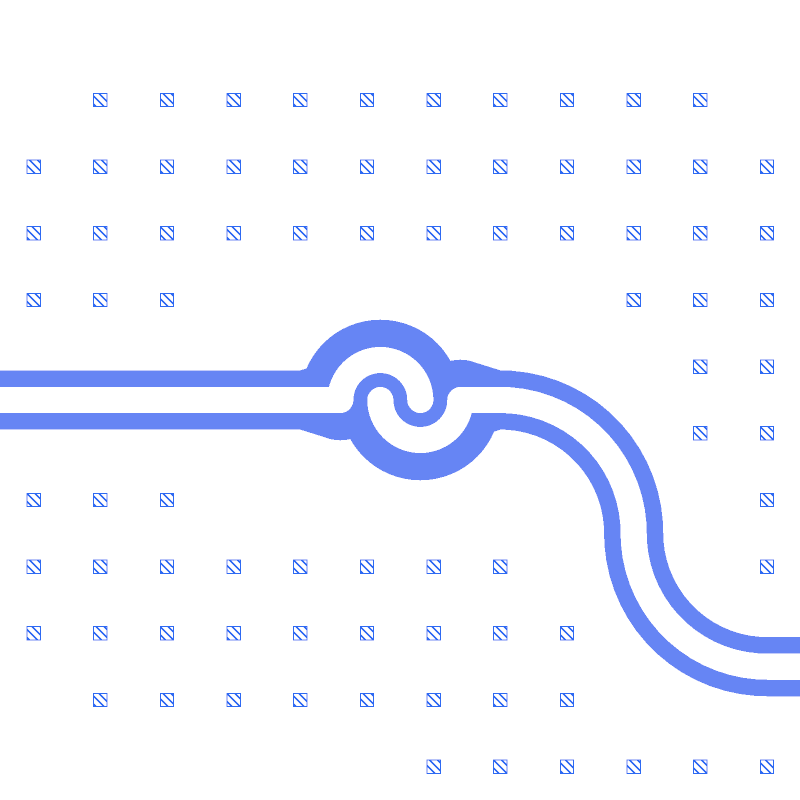
The DRC is clean. The picture shows the capacitor with its two leads (left: the route IN from the pad; right: the
route R_CAP).
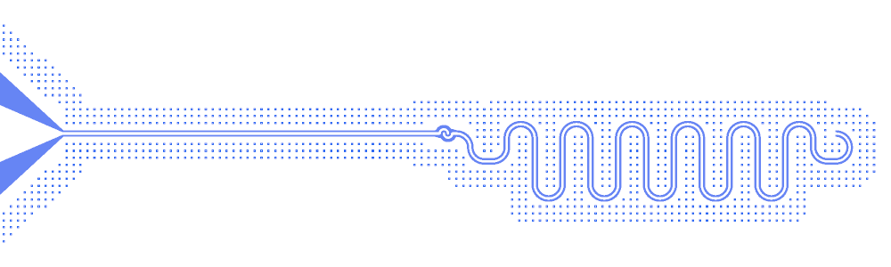
The whole chain, from the pad to the free end of the resonator:
What the LOM says
lb = d.lom(select=["PAD_IN", "C1", "IN", "R_CAP"])
res = C.simulate_lom(lb, d.design)       # C is examples/designs/_common.py
select limits the LOM to the chain. Use it whenever the chip holds a second circuit that is not connected to the
first: the normal-mode solver needs one connected network.
Branch |
Value |
|---|---|
|
27.0 fF, a rough estimate |
|
lambda/4, 4000 µm, 7.877 GHz bare |
Resonator mode with the capacitor |
7.533 GHz, kappa 41 MHz |
The number of turns sets the coupling. Each row is a rebuild and a LOM in the notebook:
Turns |
C (fF) |
f_r (GHz) |
kappa (MHz) |
|---|---|---|---|
0.5 |
11.0 |
7.731 |
7.6 |
1 |
27.0 |
7.533 |
41.1 |
1.5 |
48.0 |
7.298 |
113.8 |
2 |
75.0 |
7.031 |
236.7 |
3 |
150.0 |
6.444 |
645.7 |
These are lumped-model estimates (component formulas and calibration), not FEM results; see the LOM page for how far to trust them.
Next
The tunable resonator adds junctions to a custom component. The notebook
examples/custom_component/custom_passives.ipynb runs both pages.