A tunable resonator
A tunable resonator is a lambda/4 CPW resonator whose shorted end goes to ground through a chain of SQUIDs. A flux through the SQUID loops raises the array inductance, which lowers the resonator frequency. Use one when a resonator has to be moved after fabrication. This page builds the component in steps: the meander, the SQUID array from Quantcore trilayer junctions, the pins, the LOM model with its flux dependence, and a chip with the resonator hanging on a feedline.
The finished files are examples/custom_component/tunable_resonator.py and the notebook
examples/custom_component/custom_passives.ipynb.
What you build
Part |
Choice |
|---|---|
Class |
|
Pin |
the open end; a route connects it to a feedline hanger |
Pin |
the end of a flux-bias line next to the array (optional) |
Array |
|
LOM |
a lambda/4 line plus the array inductance, as a function of flux |
Step 1: the meander
The cell draws a zig-zag CPW of a chosen total length from pin a to the array. runs straight runs of length run
are joined by rounded corners of radius bend_radius. A rounded corner is shorter than a sharp one by
(2 - π/2) r, so the run length that gives exactly length is:
def run_length(length, runs, pitch, r, lead):
    corners = 2 * (runs - 1)
    return (length - lead - (runs - 1) * pitch + corners * (2 - math.pi / 2) * r) / runs
The path is drawn by the KQCircuits WaveguideCoplanar, which rounds the corners and draws the two gaps:
self.insert_cell(WaveguideCoplanar, path=pya.DPath(pts, 0), a=self.a, b=self.b, r=self.bend_radius)
runs must be odd, so the meander ends on the side of the array. The build stops with a message when the meander does
not fit (pitch below 2 r + a + 2 b, or a run that is too short).
Step 2: the SQUID array
The array is a chain of islands. Between two islands sits one QuantcoreSquid, the PDK trilayer SQUID of
quantcore_circuits.layouts.junctions.trilayer. The first island is the end of the CPW centre conductor; the last
SQUID lands on the ground plane.
for j in range(self.n_squids):
    x_slot_end = x_e + (j + 1) * step          # the ground side of SQUID j
    squid_trans = pya.DCplxTrans(1, 90, False, x_slot_end, y_arr)
    self.insert_cell(QuantcoreSquid, squid_trans, inst_name=f"squid_{j + 1}",
                     window_height=h, lj_nH=self.lj_nH)
The SQUID cell has its ground side at the origin and its island side at (0, window_height). The rotation by 90
degrees lays the chain along x, with the island side toward the CPW. lj_nH sizes the fingers by the PDK junction
rule: it is L_J0 of one SQUID (both junctions in parallel), and 0 draws the PDK nominal SQUID. The cell draws the
junction fingers (layers 2/0 and 4/0 in the legacy numbering, the KQC SIS_junction layers), the HSQ spacer with its
dose levels and the clearer metal that closes each gap. The pocket in the ground plane is the region around the chain
minus the islands.
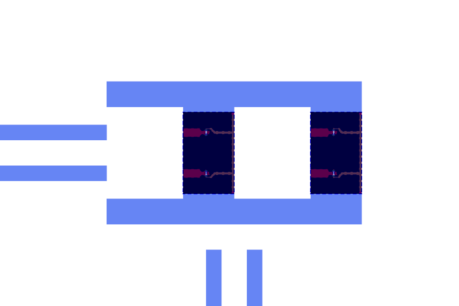
With lj_nH = 1.0 the fingers are 1.68 µm wide (the PDK maximum is 2 µm, so about 0.8 nH is the lowest L_J0 you can
draw).
Step 3: the flux line and the pins
The flux line is a short CPW that ends in a short circuit flux_gap below the pocket, so its current passes close to
the loops. Its pin points away from the array.
self.add_port("a", pya.DPoint(0, 0), pya.DVector(-1, 0))
self.add_port("flux", pya.DPoint(x_f, y_pin), pya.DVector(0, -1))
The DRC warns about a pin that no route reaches (dangling_port). Connect the flux pin to a pad, or leave it open on
purpose.
Step 4: the LOM model
The array is an inductance at the shorted end of the line. An inductance L there lowers the resonance exactly like extra line of an equivalent length. For a line of length l, phase velocity v and impedance Z0, open at one end and closed by L at the other, the resonance satisfies
tan(2π f l / v) = Z0 / (2π f L)
equivalent_length_um solves it and returns the length that a plain lambda/4 line needs to resonate at the same
frequency. The model adds that length to the line:
ej = effective_junction(inst, each, pdk, kind="SQUID")      # L_J0, flux and asymmetry of the instance
l_array = n_sq * ej.lj_eff_nH                                # N * L_J0 / sqrt(cos² + d² sin²)
extra = equivalent_length_um(l_array, geometric + route_um, a_um, b_um, pdk.name)
frag.lines.append(Line(name, "res", ("a", None), geometric + extra, a_um, b_um, ("open", "short"), True, ...))
For a symmetric SQUID (asymmetry d = 0) the array inductance is
L_array(Φ) = N · L_J0 / |cos(π Φ / Φ0)| = N · L_J / (2 |cos(π Φ / Φ0)|)
with L_J of one junction and L_J0 = L_J / 2 for the two in parallel. The flux and the asymmetry are the instance’s
junction values (flux_phi0, asym). The line has the pin a as one end (open) and the array as the other (short).
The extra length depends on the whole resonator, so the model needs the length of the route that finishes it. The
parameter route_um carries it: set it to the route length after the first build. The SQUID capacitances are not
modelled (in series they are far above the array’s reactance). The class is registered by name with
@register_lom("TunableResonator").
Step 5: register the class
As for the spiral capacitor: copy the file into src/quantcore_circuits/layouts/others/, or
layouts.register_pcell_classes([TunableResonator])
TUNE = "custom_component.tunable_resonator.TunableResonator"
Place it on a chip
The resonator hangs on a feedline. Its open end connects to a hanger whose far end is open: the SQUID array is the
short, so the hanger must not short the line as well (the default end="short" would give a lambda/2 line).
pad_w = d.add("PAD_W", "BondPad", at=(1125, 1500), rot=270, edge="auto")
pad_e = d.add("PAD_E", "BondPad", at=(6375, 1500), rot=90, edge="auto")
fl = d.route("FL", pad_w.a, pad_e.a)
tune = d.add("TR", TUNE, at=(3300, 2000))
d.route("R_TR", tune.a, fl.hanger(near=(2800, 1500), length=500, side="left", end="open"))
pad_f = d.add("PAD_F", "BondPad", at=(6375, 2900), rot=90, edge="auto")
d.route("FLUX", tune.flux, pad_f.a)
d.show()
tune.set(route_um=d.result.route_lengths()["R_TR"])   # 1636 µm here
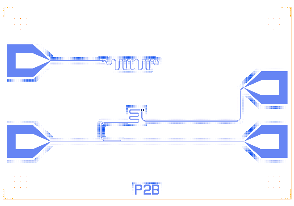
The DRC is clean. The zoom shows the meander, the array and the flux line below it:

The whole chip (the upper circuit is the capacitor chain of the spiral capacitor page):
What the LOM says
lb = d.lom(select=["PAD_W", "PAD_E", "FL", "TR", "R_TR"])
tune.set(junction={"flux_phi0": 0.3})
d.show()
res = C.simulate_lom(d.lom(select=[...]), d.design)
The builder note reads TR: 2 SQUIDs, L_array 2 nH at Phi = 0 Phi0 (L_J0 1 nH each) = 3460 um of extra line at the shorted end. The resonator is a lambda/4 line of 6496 µm equivalent length with a hanger coupling of 0.197 MHz.
Flux (Φ0) |
L_array (nH) |
f_r LOM (GHz) |
f_r QuCat (GHz) |
|---|---|---|---|
0 |
2.00 |
4.851 |
4.825 |
0.1 |
2.10 |
4.753 |
4.728 |
0.2 |
2.47 |
4.445 |
4.423 |
0.3 |
3.40 |
3.874 |
3.857 |
0.4 |
6.47 |
2.891 |
2.882 |
0.45 |
12.78 |
2.091 |
2.086 |
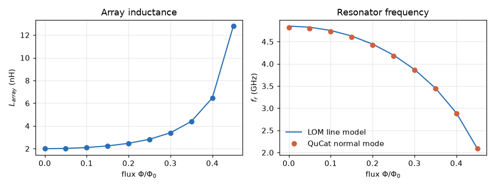
The frequency falls as |Φ| grows, from 4.83 GHz at zero flux to 3.86 GHz at 0.3 Φ0. The 1 nH per SQUID is the smallest
inductance the PDK junction rule can draw, so this array tunes strongly. Use a shorter length for a higher
starting frequency, or more junctions of a smaller L_J0 for a smaller swing. These are lumped-model estimates
(component formulas and calibration), not FEM results; see the LOM page for how far to trust them. The
mutual inductance of the flux line to the loops is not modelled: the flux is a design value.