The Flow strip
The Flow strip is the row of six buttons at the top of the Quantcore panel. It walks a design through the flow: Design, Check, LOM, Simulate, Results, Fab. Use it once the chip is drawn, to check it and send it to the fab. Each button runs the matching menu action, and a mark on it shows the state of that step.
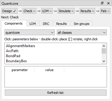
The panel after Open: Design is done and the line under the strip names the next step.
Reading the marks
Mark |
Meaning |
|---|---|
✓ |
Done |
⚠ |
Done, but out of date or with issues |
– |
Not done yet |
The line under the strip names the next step. A step goes out of date when the design changed after it ran: Check and LOM when the design changed, Simulate when the results belong to another revision, Results when a target fails, Fab when the mask is older than the design. Writing a sim group or a target does not make a step out of date.
The six steps
Step |
Menu item |
What it does |
Where you see it |
|---|---|---|---|
Design |
Design menu |
Draw the chip (place and route) |
The layout |
Check |
Check and LOM > Check design (Ctrl+Shift+D) |
Design checks: dangling ports, overlaps, crossings, opens and shorts |
DRC tab |
LOM |
Check and LOM > Run LOM simulation (Ctrl+Shift+O) |
Lumped circuit of the chip, solved with QuCat and QuTiP |
LOM tab |
Simulate |
Simulate menu |
Full-wave or FEM run of selected components |
Results tab, status bar |
Results |
Results menu |
Values against targets, and Propose next revision |
Results tab, windows |
Fab |
Fab menu |
Mask, netlist, |
A folder, |
Check
Check design (Ctrl+Shift+D) runs in the background and fills the DRC tab with errors, warnings and PDK design warnings. Click a line to zoom to its marker.
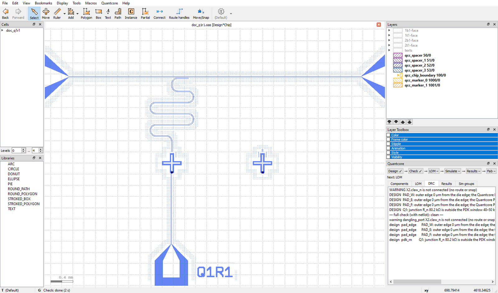
After Check. X2.claw_n is a dangling port. The pad_edge warnings come from pads that sit at the default position.
Fix pad edge warnings (Check and LOM menu) sets place.edge = "auto" on every pad the PDK pad rule flags. The
build then slides the pad perpendicular to the nearest die edge until its outer etch edge is 100 µm from it. The rules
are listed on routing and DRC.
LOM
Run LOM exports the circuit (build/<name>.circuit.json) and simulates it in a background process. The LOM tab
shows the modes, f_q, α, f_r, χ and κ against your targets, the netlist values and a picture of the circuit.
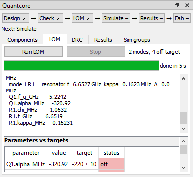
The LOM tab after Run LOM.
A progress bar shows the stage (export, read, QuCat and QuTiP, write, draw) and the elapsed time.
Stop (next to Run LOM) kills only the LOM process this panel started and restores the tab as it was.
The run stops by itself after the time limit (Settings > Run LOM time limit, default 30 minutes).
Run LOM always solves the whole chip in one network. On a big chip it can take longer than the limit.
A value is within tolerance by the same rule as
qcc analyse: f_q ±20 MHz, f_r ±10 MHz, α ±10 MHz, g ±10 MHz, χ ±0.1 MHz, κ ±0.2 MHz, any other key ±1 %.A qubit with no junction value gives an open circuit. Set L_J in the component dialog first.
The circuit picture opens in its own window with the buttons Fit, 100 %, − and +. How far to trust the numbers: the LOM page.
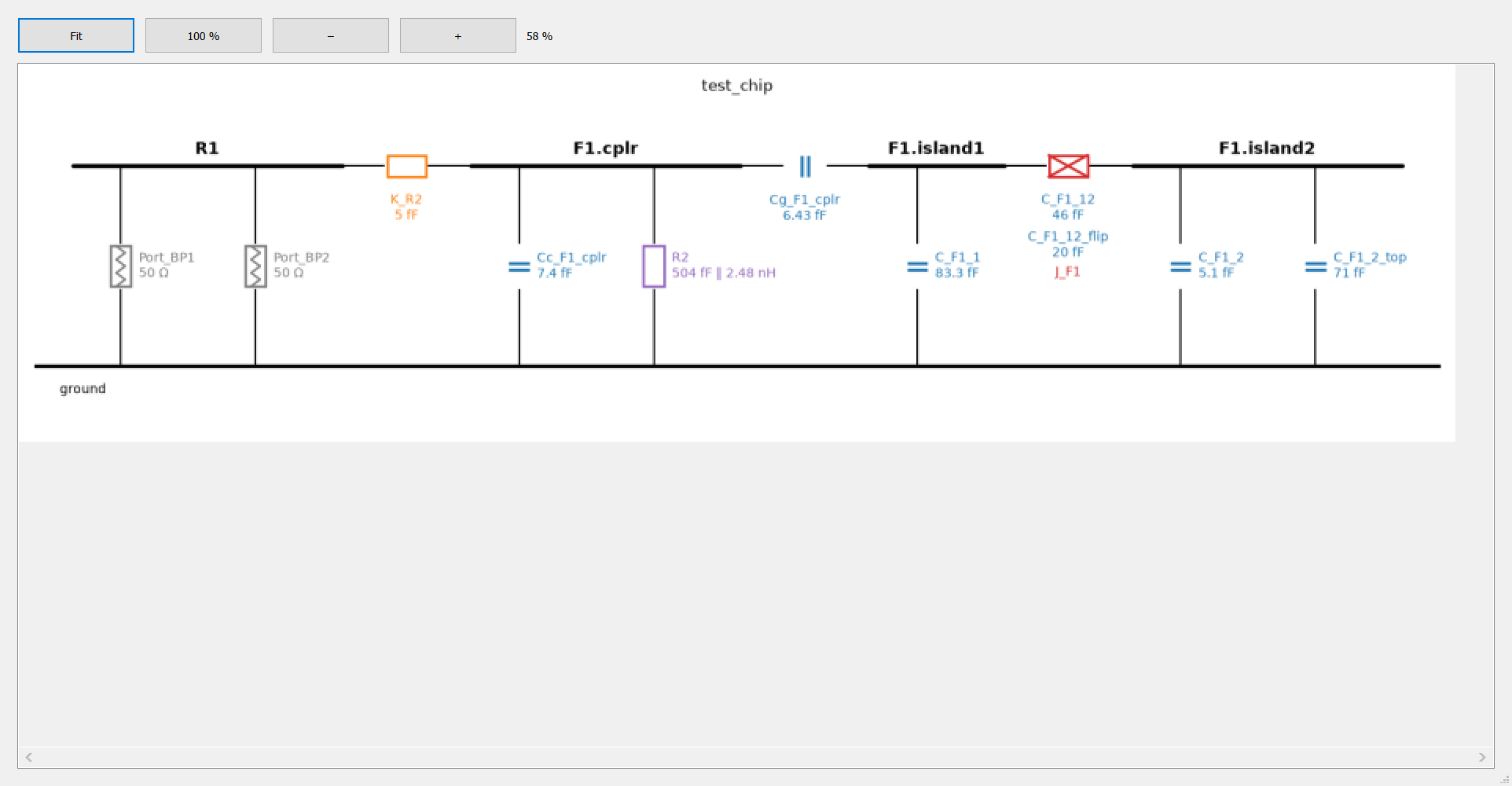
The circuit picture window.
Simulate
Simulate selected components runs a full-wave or FEM solve of the components you select with KLayout’s Select tool. Nothing selected: it offers the default subset (the first qubit with its readout) or the whole chip, which is slow and needs a lot of memory. The Simulate dialog opens first.
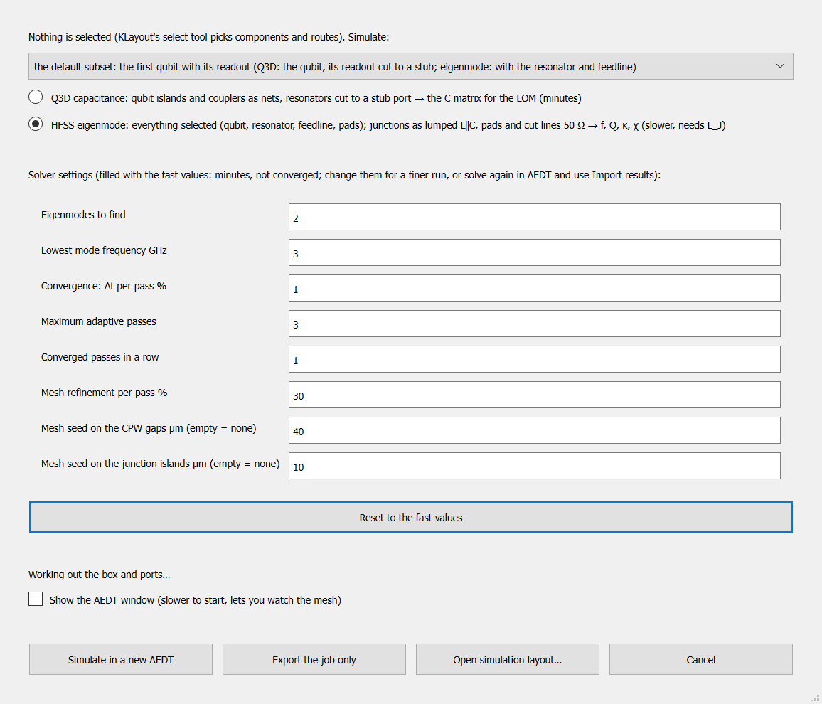
The Simulate dialog.
Analysis |
What it renders |
Chosen when |
|---|---|---|
Q3D capacitance |
The selected qubits’ islands and couplers as nets; resonators cut to a stub port |
You select qubits only |
HFSS eigenmode |
Exactly the selection, junctions as lumped L‖C, pads and cut lines 50 Ω |
You select a line, a resonator or a pad, or nothing |
An eigenmode run needs L_J on every junction. If one is missing, the run and export buttons are disabled, and the warning names the component and where to set it (component dialog, junction section).
The dialog also holds the solver settings, filled with fast values and kept for the next run (Reset to the fast values). The plugin is for quick prototyping: driven and full-wave S-parameter runs are for scripts.
Buttons:
Simulate in a new AEDT: runs
qcc sim autoin the background. It exports the job, solves it in a new non-graphical AEDT (tick the box for a visible window), then analyses it. The AEDT you have open is never attached to or closed. KLayout stays usable and the status bar shows the progress. A small qubit and readout box takes about a minute. Pressing Simulate while one runs offers to stop it.Export the job only: writes the job folder (geometry, AEDT scripts,
job.json,results_template.json, a README with what to run and what to bring back). Solve it by hand or on another machine.Open simulation layout: shows in a new tab the geometry AEDT would import, with readable layer names and the port polygons. No AEDT is started and the design is untouched. Closing the tab asks to save the in-memory port layers; answer No.
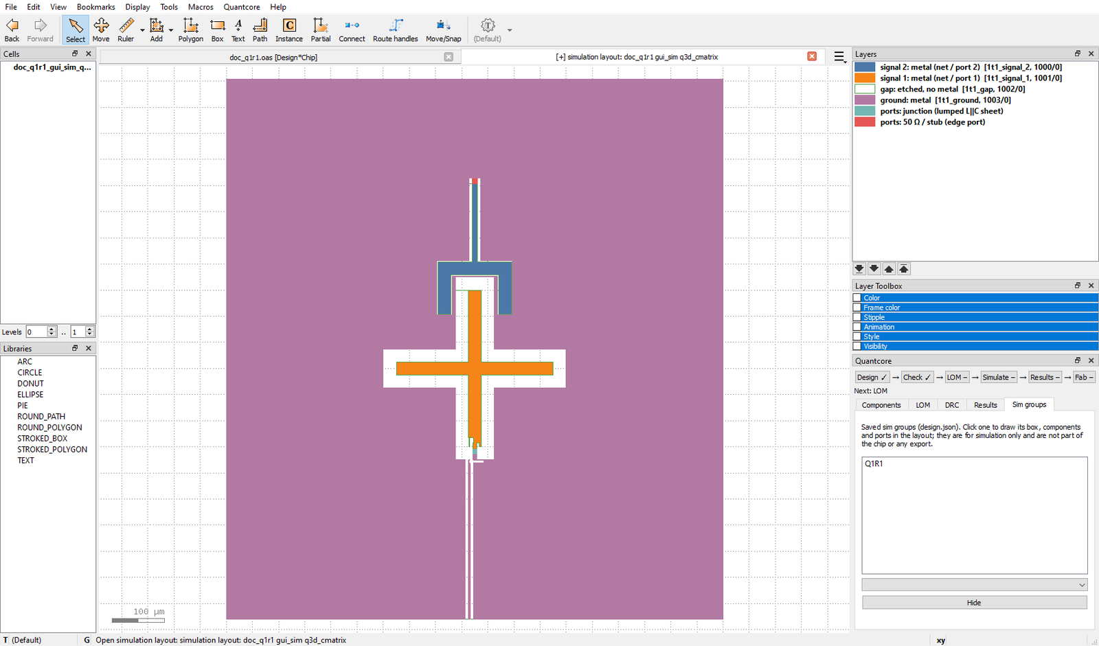
Open simulation layout: the exported geometry in its own tab.
A run started with Simulate outlives KLayout. When you reopen the design, a run that ended meanwhile is imported at once, and one still going is imported when it ends.
Import results
Import results… (Simulate menu) takes a solved job folder or a results.json file. The values are checked against
the design (net names, matrix shape) and analysed. qcc results template DESIGN writes a skeleton with your net names;
qcc results template --format prints the format. The command-line equivalents are qcc sim subset, qcc sim auto
and qcc results import; see the simulation page.
On Windows keep the AEDT job folder path under about 140 characters. A deeper design folder makes the automatic run use
%TEMP%\qcc_jobs.
Warning
Eigenmode from the Simulate dialog, --aedt gui from the plugin and a whole-chip simulation from the GUI have not been tested.
The test ran Q3D of one qubit in a new non-graphical AEDT. See status.
Results and tune
Results against targets… shows the latest values, the same rows as the Results tab. Values from an older revision are marked stale.
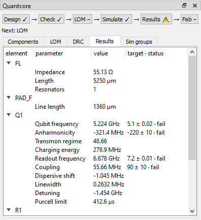
The Results tab: each value with its target and pass or fail. This result file belongs to a different design, so the numbers show how the tab works, not a real simulation of this chip.
Propose next revision… is the tune step. It reads the last simulation (or the layout’s LOM estimates) and previews the old and the proposed knob values: L_J for f_q, the qubit’s island knob for α, its coupler knob for g, the resonator length for f_r. Only knobs whose target is set move. What cannot be tuned (a junction without L_J, a readout drawn as a plain route, a qubit with no readout) is listed under Not tuned.
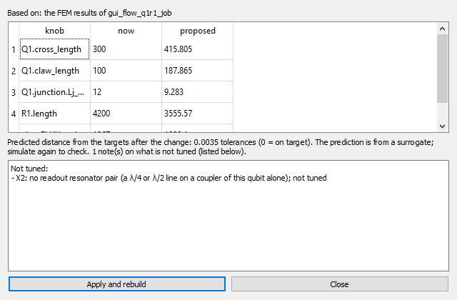
The proposal window: knobs now and proposed.
Apply and rebuild writes the values to design.json as one undo step and rebuilds. The LOM, Simulate and Results
steps then show as out of date. Simulate again to check the result.
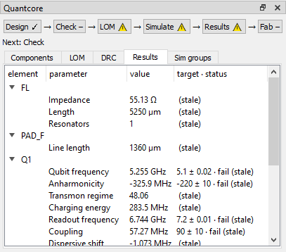
After Apply: LOM, Simulate and Results are out of date, and the old results are marked stale.
The tuning knobs per qubit class are listed in the docstring of src/quantcore_circuits/codesign.py. The tune step is
described further in the feedback page.
Fab
Export for fab… writes into one folder (default build/):
File |
What |
|---|---|
|
The negative mask on the Quantcore fab layers, with the PDK frame, the 100 µm pad rule, the cheese band and corner rounding |
|
The netlist |
|
The drawn chip as a Designer script that writes the same |
a PNG |
A picture of the mask |
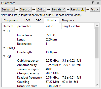
The panel after Export for fab: Fab is done.
The export refuses while a route has failed. Design > Save as Python script… writes only design.py, so a GUI
prototype can continue as code (scripted design). The mask rules are on the fab page.
Values on the layout
The Values tab shows, for every qubit and resonator, the LOM value, the FEM value (once a field solver result is imported), the consensus with the spread between methods, and the target with its tolerance. Qubits show f_q and α, resonators f_r, κ and χ. Tick Show values in the layout and the same values are written beside each instance, coloured by |value − target| / tolerance:
Colour |
Meaning |
|---|---|
Green |
Within the tolerance |
Amber |
Up to twice the tolerance |
Red |
Further off |
Grey |
No target to compare with |
The colour judges the FEM value when there is one, else the LOM value, else the consensus. Select an instance with
KLayout’s select tool and the tab reads out its values; click a row of the tab and that instance is selected and
shown. The values refresh after every rebuild, Run LOM and Import results. They are drawn as markers and never
written to design.json or the layout.
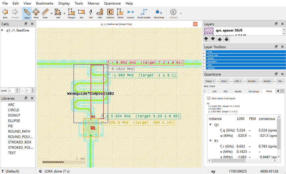
The Q1 + R1 chip after Run LOM, with the toggle on. Here the targets are set so that all three colours show.
Settings that matter here
Setting (Quantcore > Settings…) |
Why |
|---|---|
qcc executable |
The |
Run LOM time limit (minutes) |
When Run LOM stops by itself |
Instance name labels: height µm |
Height of the names on the |
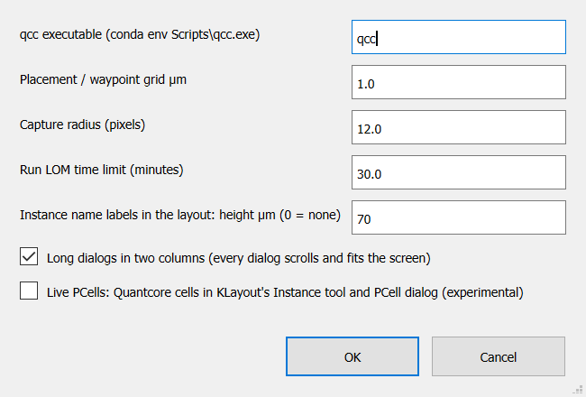
The Settings dialog.