EPR from the LOM and eigenmode runs
Energy participation ratio (EPR) turns a linear circuit into the Hamiltonian of its junctions: for each mode m and
junction j, p_mj is the fraction of the mode’s inductive energy that sits in the junction. From the p_mj and
the linear mode frequencies you get the dressed frequencies, the anharmonicity α, the cross-Kerr (dispersive) shifts
χ and the Lamb shift of every mode. Use it when you have eigenmode frequencies or a LOM and want these numbers
without a field integral.
Junctions in a Quantcore layout are lumped inductors (L_J, plus C_J). That is what makes the field integral of
pyEPR unnecessary: the participation can be read off how a mode frequency moves with L_J, or taken from the LOM.
The code is quantcore_circuits.analysis.epr_lumped; the field-integral path (analysis/epr.py, run inside AEDT)
stays as it was.
The three routes
Route |
|
Input |
Cost |
Good for |
|---|---|---|---|---|
Eigenmode |
|
eigenmode frequencies of the nominal solve and of solves with one junction’s |
one extra eigenmode solve per junction and step |
qubit modes and any mode with |
LOM |
|
a LOM result (QuCat normal modes) |
none |
every mode; the first estimate, before any FEM |
Energy |
|
peak junction current and total energy, or a job that holds pyEPR’s |
the field export |
the check for the other two |
All three return the same dictionary and use the same standard EPR formulas for what follows
(epr.epr_hamiltonian: phase zero-point fluctuation from p_mj, the cosine expanded, numerical diagonalisation).
Eigenmode L_J sensitivity
For a mode with frequency ω the energy in the junction inductance is what moves the frequency when L_J changes
(Hellmann-Feynman):
For a junction in series with other inductance in one LC mode this is exactly L_J / L_total. Solve the eigenmode
problem at the nominal L_J and with each junction’s L_J changed by about ±2 %; the other junctions and the mesh
stay as they are.
from quantcore_circuits.analysis import epr_lumped as L

res = L.eigenmode_dL(
    "fem/t04_ALL_eigenmode",             # nominal solve (results.json, job folder, or a list of GHz)
    lj_nH=[7.32, 6.475],                 # nominal L_J of Q1 and Q2
    perturbed={                          # one junction changed per solve
        "Q1": [(7.32 * 0.98, "fem/q1_m2"), (7.32 * 1.02, "fem/q1_p2")],
        "Q2": [(6.475 * 0.98, "fem/q2_m2"), (6.475 * 1.02, "fem/q2_p2")],
    },
    junctions=["Q1", "Q2"],
    labels=["Q1", "Q2", "R1", "R2"],
)
With three or more points (nominal plus two) the slope comes from a quadratic fit in ln L_J; with one perturbed
solve it is the plain finite difference (at the mid-point of the step). The result carries a note when the step is
below 0.05 % or above 10 %, when modes changed order, or when the participations of a mode add up to more than 1.
From the LOM
from quantcore_circuits.analysis import epr_lumped as L

res = L.epr_from_lom(lom)   # lom: the LOM result (lom.simulate.simulate, Designer.simulate)
The LOM’s QuCat network already stores each mode’s inductive energy per element, so the participations come directly from it. The result is only as accurate as the LOM’s component estimates (see the LOM page).
From the field energy
res = L.epr_from_energy(f_GHz, lj_nH, i_peak_A, u_total_J)          # p = 1/2 L_J I^2 / U
res = L.epr_from_job("fem/t04_ALL_eigenmode/results/results.json")  # the participations pyEPR recorded
The result
epr_result builds one dictionary for all three routes:
Key |
Content |
|---|---|
|
|
|
list of |
|
the junction names |
|
|
|
self-Kerr of each mode (negative for a transmon) |
|
M × M matrix: α on the diagonal, cross-Kerr off it |
|
dressed minus linear frequency |
|
the linear and dressed frequencies, the inputs, caveats |
Modes whose largest participation is below 1e-4 are left at their linear frequency. The numerical diagonalisation
has dimension fock ** modes, so it runs for the four modes with the largest participation; the others get the
first-order values, and a note says so.
s_mj is the relative sign of a junction’s phase in a mode. The dL and LOM routes give only |p|, so it defaults
to +1. It matters only when one mode touches two junctions (the cross-Kerr between them).
epr_md(res) prints a result as tables. compare_epr(a, b) and compare_md(a, b) line two results up mode by mode
(for example lom against eigenmode-dL): frequency, largest participation and α of each, and the difference.
How accurate
Measured on a transmon (9 nH, 85 fF) coupled to a resonator, where the exact participation is known:
What |
Result |
|---|---|
|
error in |
|
1.4 % error of the weak mode; the error is about 0.7 times the step |
|
|
|
|
|
within 5 % (tested on the Q1 / R1 example) |
The noise rows are the practical limit. The adaptive mesh of separate eigenmode runs makes frequencies differ by
1e-4 to 1e-3 between runs, so the dL route cannot resolve the 1e-3 participation of a readout resonator in a
qubit-dominated pair of modes; it resolves the qubit mode and strongly hybridised modes well. Reuse the same mesh for
all solves of a junction scan (no adaptive passes), and take the weak participations from the LOM or the field
energy. The kept two-qubit job shows the scale: p of the qubits is 0.985, of the resonators 5e-4, and the
dispersive shifts that follow are 0.16 to 0.24 MHz.
Plots
plots.plot_epr(res) draws the participation bars per mode and junction (log scale) and the χ matrix (signed, with
the values printed). In a notebook, epr_lumped(...) from examples/designs/_common.py shows the tables and the plot
in one call; eigen_md(keep) also shows the plot for a kept job that has EPR values.
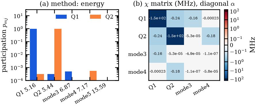
EPR of the kept two-qubit eigenmode job (tutorial 4): the participations of Q1 and Q2 per mode, and the χ matrix with α on the diagonal (about -150 MHz each) and the 0.2 MHz dispersive shifts to the resonator modes.
The same result reaches the dashboard: plots.epr_specs(res) gives a participation bar plot and a χ heatmap for the
Plots tab (dashboard).