LOM
The LOM (lumped-element model) gives a first estimate of a chip’s frequencies without a field solver. Use it to check a design in seconds, to size a qubit and readout before drawing them (LOM first), and as the frame into which solver results are later filled. The estimates come from component formulas and calibration, not from FEM; see the limits at the end.
The layout becomes a circuit as follows. Each component has a model that maps its ports to nodes and branches (capacitances, junctions, lines); routes become conductors or resonators; the pieces are merged into one whole-chip netlist, which is then solved.
lb = d.lom()                                   # layout -> LOM netlist (values = component estimates)
res = simulate_lom(lb, d.design)               # QuCat normal modes + kappa, QuTiP dressed spectrum
d.lom() is lom.lom_from_design; the simulation is lom.simulate.simulate() returning a LomResult. From the
command line: qcc circuit export DESIGN writes circuit.json, and qcc circuit simulate CIRCUIT [--json --png] runs
it. In the plugin it is Run LOM (Ctrl+Shift+O).
What it writes
qcc circuit export DESIGN writes build/<name>.circuit.json; Designer.lom() returns the same netlist in memory.
Results are printed as tables and drawn in the circuit window and the dashboard.
Tutorial 0, one qubit with a lambda/4 readout (sections 7 and 8):
4 nodes, 8 branches, 0 controls, 0 unconnected ports
| C_Q1 | C | Q1 - gnd | 96.1 fF |
| J_Q1 | JJ | Q1 - gnd | Lj 6.87 nH, Cj 14.7 fF |
| R1 | TLres | Q1.claw_n - gnd | lambda/4, 4501 um, 7.000 GHz |
| K_R1 | HANGER | Q1.claw_n - FL | kappa 0.214 MHz (L 300 um) |
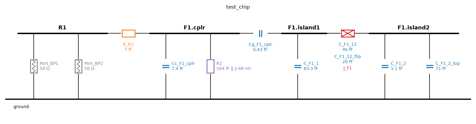
The circuit drawing (circuit/draw.py, qcc circuit simulate --png; also the plugin’s circuit window): feedline,
resonator, coupling capacitors and junction as one schematic.
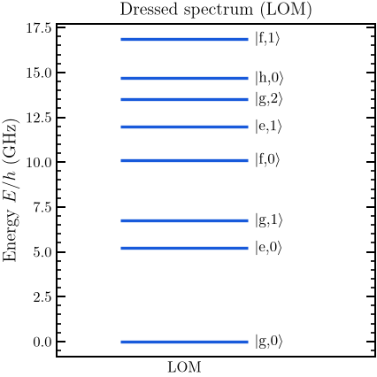
LOM dressed spectrum from examples/lom_from_layout.ipynb: the lowest states of the qubit and resonator.
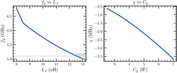
Sweeps on the LOM from the same notebook: qubit frequency against junction inductance, and the dispersive shift chi against the qubit-resonator coupling capacitance.
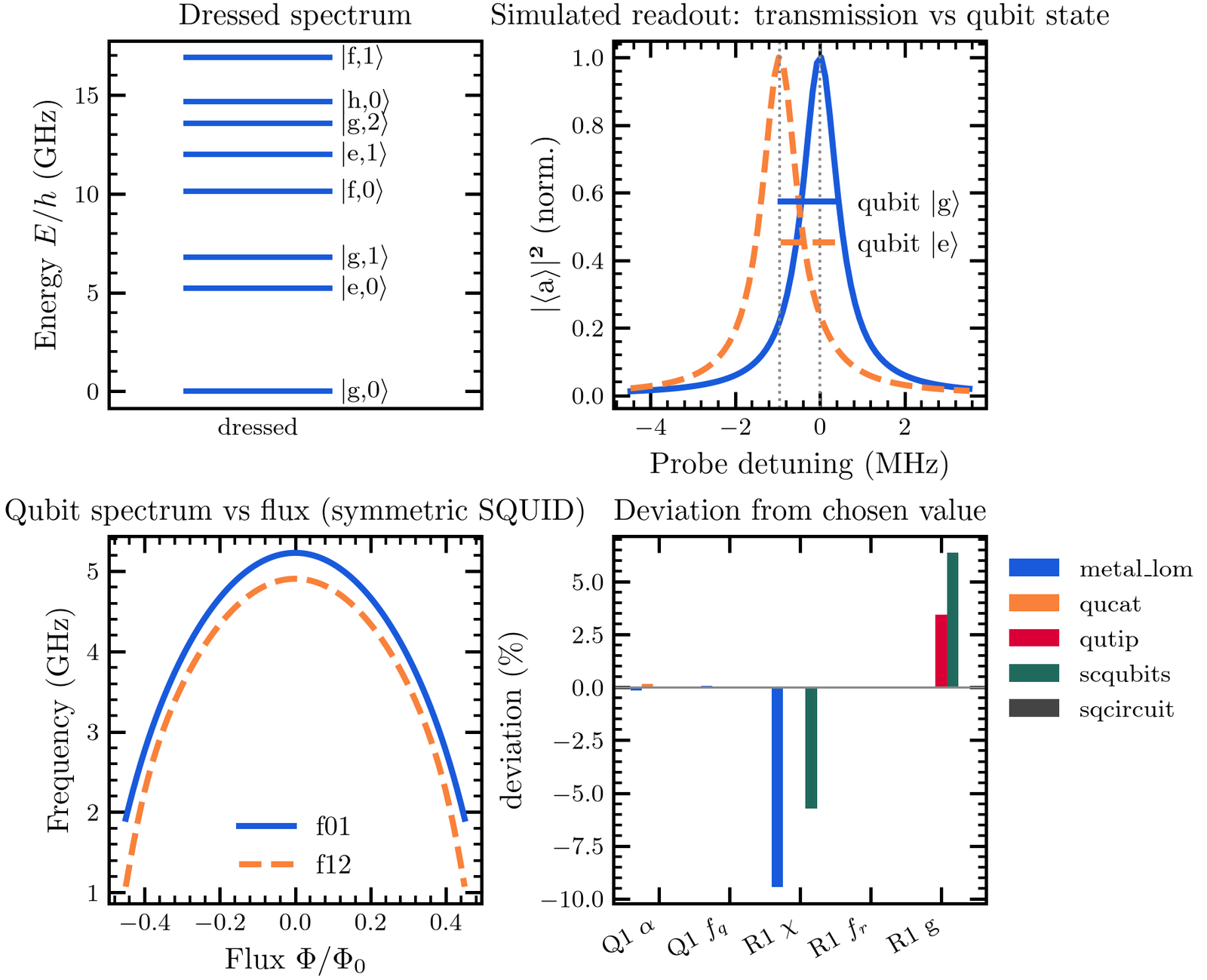
The four panels the dashboard also shows (dressed levels, simulated readout, flux curve, estimator spread), here for the Q1 / R1 feedline example (an older render).
Estimators: metal_lom, qucat, sqcircuit, scqubits, qutip and pyepr (when an eigenmode result exists);
circuit/consensus.py picks one value per parameter and flags the spread. Agreement with SQcircuit is 0.1 % on f_q and
1 % on alpha for the check circuits.
LOM first: targets to layout
qcc synth --f-q --alpha --f-r --g solves L_J, C_sigma, C_g and the lambda/4 length for one qubit and readout.
lom.synthesize.layout_from_targets and qcc circuit layout CIRCUIT -o OUT --live draw the chip.
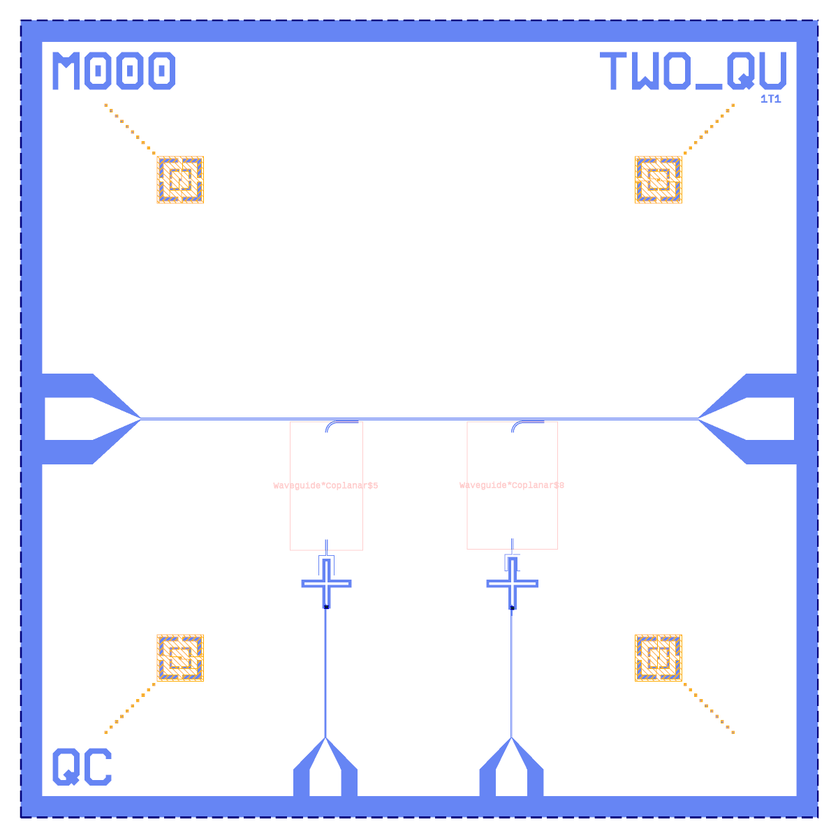
Two qubits laid out from targets (examples/lom_from_layout.ipynb): two Xmons, two lambda/4 readouts on one feedline,
DRC clean. Only the Xmon with a lambda/4 readout on one feedline is supported; other topologies are not built.
Limits and known gaps
A pin that is not connected is not kept floating: tutorial 3’s Run LOM fails with “open or shorted”.
QuCat hits its recursion limit at 8 junctions; whole-chip LOM of a 21-qubit chip does not finish on this PC (9 min, 4.7 GB). The LOM stays whole-chip; run it on a bigger machine.
TransmonCross claw capacitances are off (claw-to-ground C about 2x low),
HANGER_Kuses one coupling constant for all hangers (lambda/4 kappa about 35 % low, open lambda/2 about 5x low), and the Purcell filter between series capacitors is not loaded.The SQUID static flux bias is dropped in
lom/simulate.py.
See status for the ranked list.