Results and plots
After a solver has run, this is how its output becomes numbers you can compare with the design’s targets: one
results.json per job, a filled circuit, tables and plots. Use it to import results solved elsewhere (a server, a
colleague), to check convergence, and to draw the figures. It writes results/results.json inside the job folder.
Read-back
analysis/results.collect_results(job_dir) turns solver output into one results/results.json: the Maxwell C-matrix with
net labels, eigenmodes, EPR, convergence and S-parameters with notch fits. Helpers: parse_cmatrix_json, parse_eig,
parse_convergence, parse_touchstone, fit_notch, fit_notches, fem_kappa, combine_jobs.
Command |
What it does |
|---|---|
|
Parse the solver outputs in a job into |
|
Read solved results back (a job folder, its |
|
A |
|
Extract Hamiltonian parameters and compare with targets; print stored results |
|
Re-export a solved project as it is now (no solve) |
Note
qcc results import (the plugin’s Import results) can rewrite results/results.json inside the job folder you give it
when it collects from raw files. Import from a copy of a fixture, not from tests/data.
circuit.fill.fill(model, design, jobs) puts the FEM values into the LOM (only the components each job owns); estimate,
FEM and design values stay side by side. In the tutorials T.solve_or_load, T.kept_results and T.kept_matches load
kept results.
What it looks like
The tutorials print each result as a table (tutorial 4, kept FEM results, fast settings):
| analysis | passes | tets (last) | criterion | last delta / target | converged | wall time (s) |
| q3d_cmatrix   | 8 | 10314  | Delta %           | 2.34 / 2.0   | False | 40.6  |
| eigenmode_epr | 3 | 249330 | Max Delta Freq. % | 2.77 / 1.0   | False | 994.2 |
| hfss_driven   | 4 | 297344 | Max Mag. Delta S | 0.0182 / 0.05 | True  | 661.7 |

| mode | f linear (GHz) | Q | p_J | f dressed, pyEPR (GHz) | self-Kerr (MHz) |
| 1 | 5.5342 | 1.215e+06 | 0.9872 | 5.3613 | -180.3 |
The C-matrix, eigenmode and notch tables follow the same pattern (T.cmatrix_md, T.eigen_md, T.driven_md,
T.convergence_md).
Plots
Library plots follow the project plot style (plots.py: use_style, figure, xy_spec, bar_spec, levels_spec,
heatmap_spec, plot_spec, save). A PlotSpec is a dict drawn by both matplotlib and the dashboard.
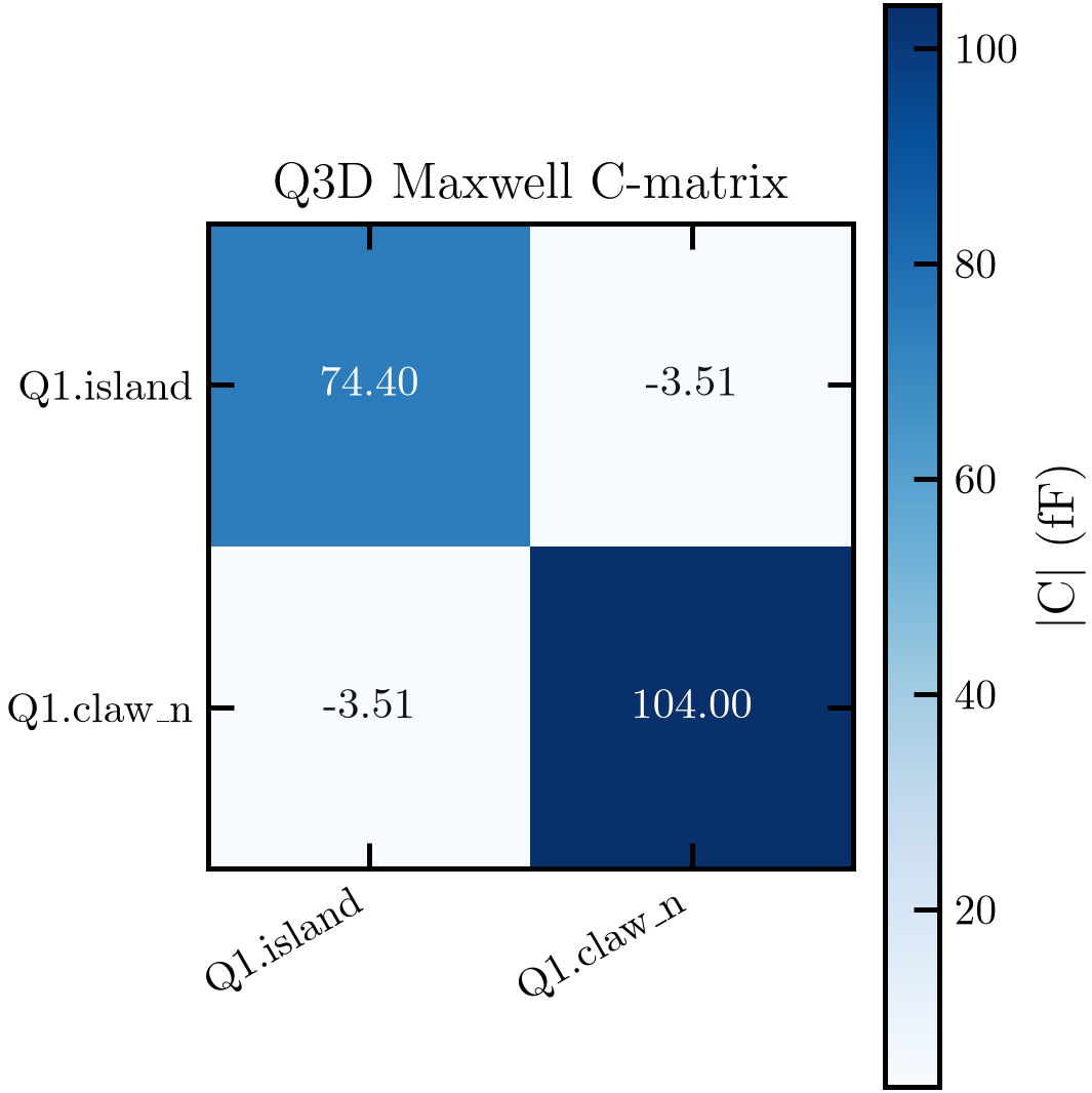
Maxwell C-matrix heatmap of the Q1 / R1 Q3D job: island and claw, in fF.
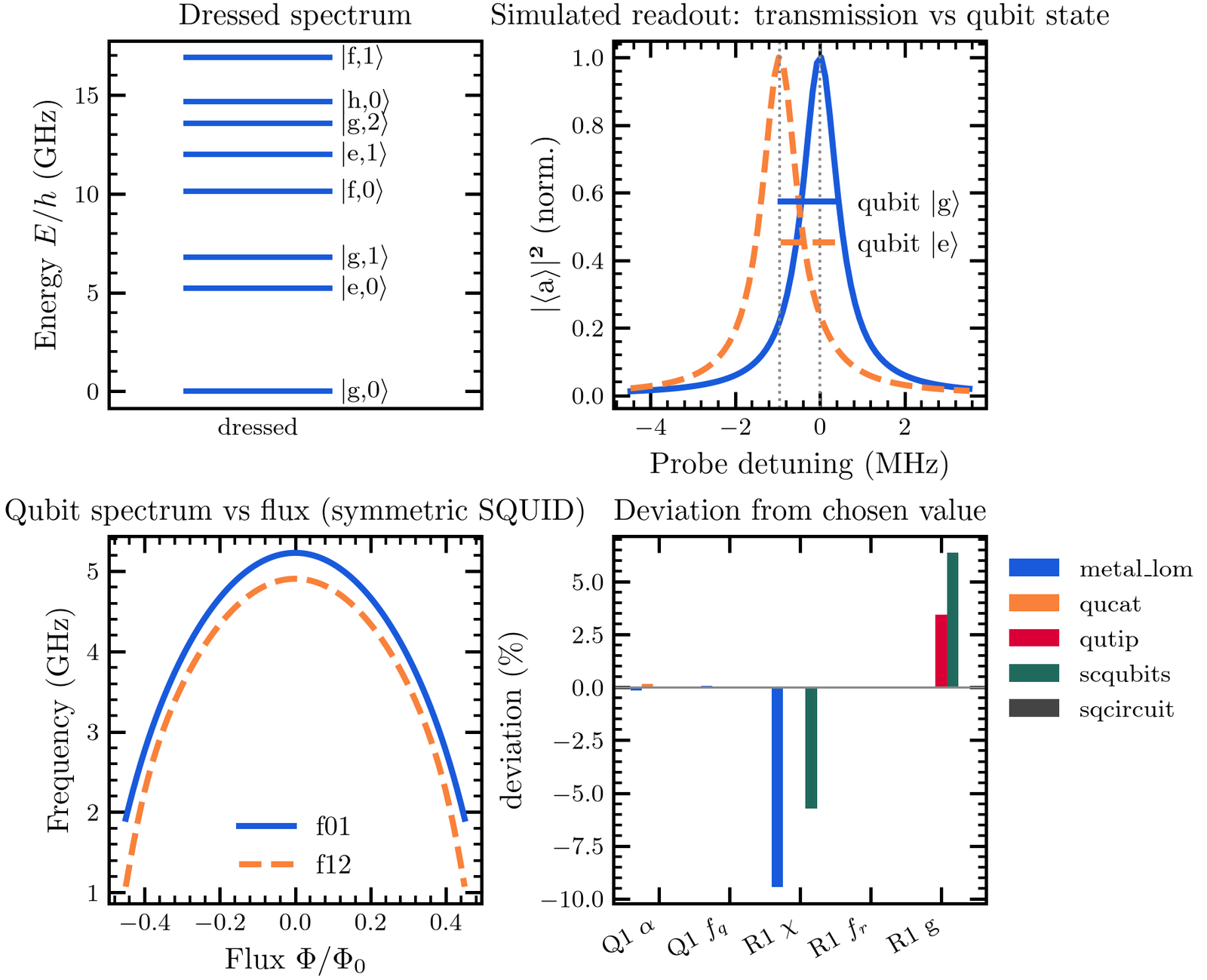
Hamiltonian panels: dressed spectrum, simulated readout, qubit frequency against flux, estimator spread.
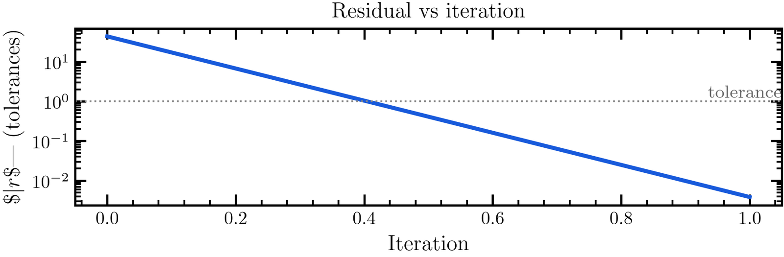
Residual against tolerance by iteration of the emulated loop on the Q1 / R1 example.
Convergence
plots.plot_convergence(results) draws the adaptive-pass convergence of a job from results.json["convergence"] (or
a job folder, or the *_project_convergence.txt): the criterion per pass with its target as a dotted line, the same
against the number of solved tets, and for an eigenmode job each mode’s frequency per pass relative to the last. Several
jobs with different criteria are drawn as Δ / target, so the line at 1 is the criterion for all of them.
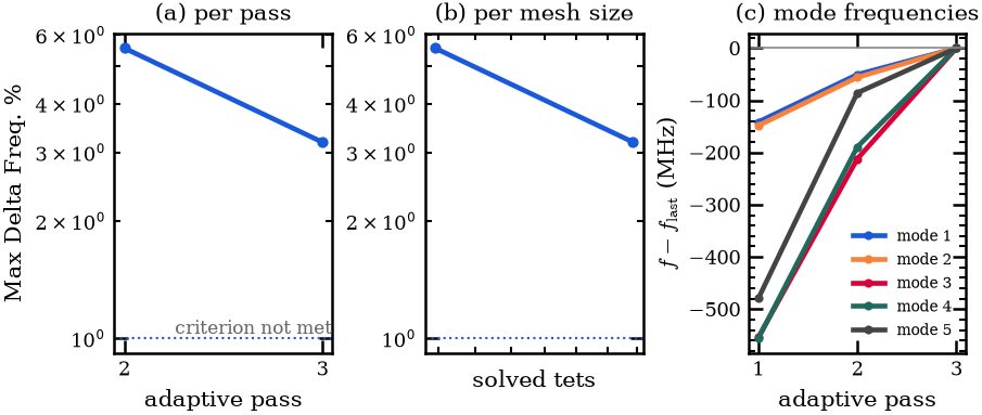
Eigenmode job of tutorial 4 (fast settings): the maximum Δf is 3.2 % after three passes, target 1 %. Modes 3 to 5 move by 80 to 200 MHz between the second and the last pass, so the frequencies are not converged.
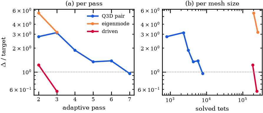
Q3D, eigenmode and driven jobs of tutorial 4 as Δ / target. Only the Q3D job (pass 7) and the driven job reach 1.
S21 and its notch fit
plots.plot_s21_fit(results) draws |S21| with the notch fit and writes f₀, κ_ext and Q_i on the panel. The trace
itself is not in results.json (only the fit), so a kept job shows the fitted curve alone; give it a job folder with
the raw *_SMatrix.s2p (or f_GHz / s21) to see the data and re-fit it.
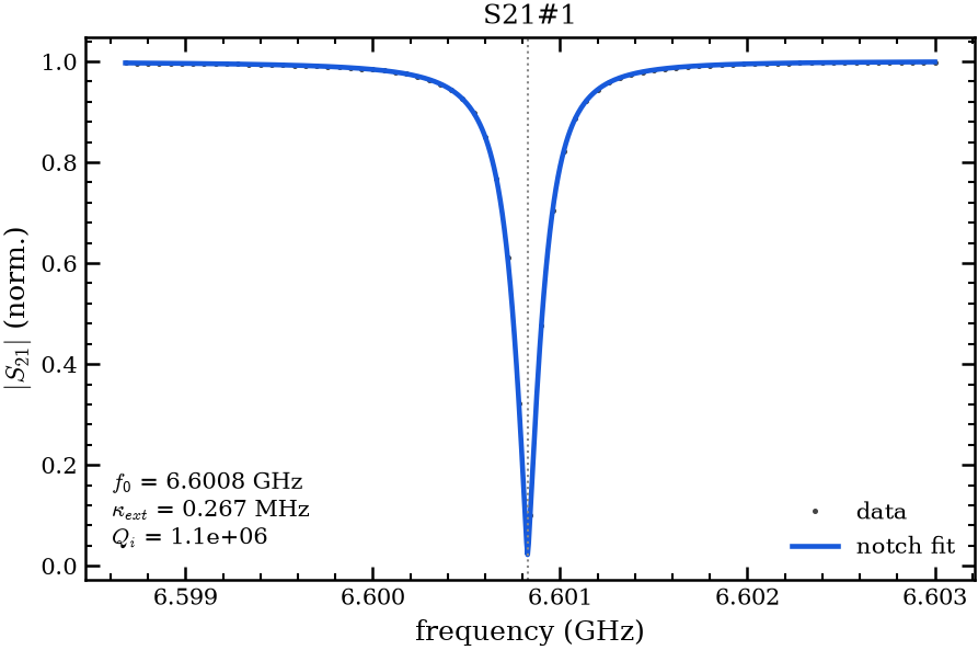
|S21| of the real AEDT 2024 R1 driven solve in tests/data/aedt_2024r1/hfss_driven (data points) with the notch fit.
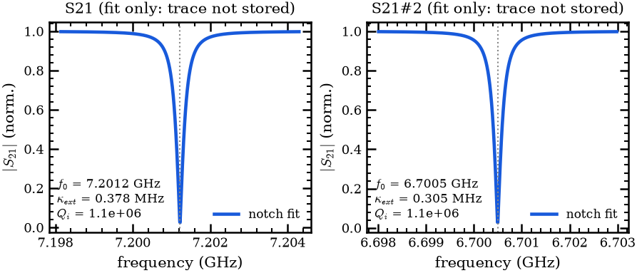
The two notches of the kept tutorial 4 driven job: the fit only, because the kept results store no trace.
EPR
plots.plot_epr(res) draws the participations and the χ matrix of an EPR result; see EPR.
In the notebooks and the dashboard
In the design notebooks convergence_md(keeps), driven_md(keep) and eigen_md(keep) show the matching plot next to
their table. The helpers plot_convergence, plot_s21_fit, plot_epr and epr_lumped in
examples/designs/_common.py can also be called on their own.
For the dashboard, plots.fem_specs(jobs) turns the solved jobs into PlotSpecs: convergence per pass and against the
mesh, the mode frequencies per pass, the S21 notches (with the data when the trace is available) and the EPR
participations and χ matrix. loop.analyse adds them to the run, so they appear in the Plots tab when a run has
eigenmode, driven or Q3D results. The React app draws any PlotSpec.
Gaps
Elmer and Sonnet results have no reader. results.json keeps no S21 trace, only the fit (add the raw trace to
collect_results if the dashboard should show the data for kept jobs). The fixed-mesh L_J scan that the dL route
needs is not a job type the exporter writes yet: the perturbed solves are made by hand (change the junction’s
inductance, solve again).