Feedback
Feedback turns solver and LOM values into new geometry (a junction inductance, a resonator length) and writes the
next revision of the design. Use it when a result misses its target and you want the library to suggest the change
instead of tuning by hand. It writes a proposal and a new design.json revision; nothing changes until you apply it.
Only one tutorial runs the loop with real FEM results; see the end of the page. The steps are:
FEM and LOM values go into one consensus against the targets (
loop.analyse(design, jobs)returns anAnalysiswith rows, estimates, plots and cards).A surrogate (least squares on the knobs, calibrated by
lom.calibration) proposes new knob values (loop.feedback(an, design_source=...)returns the proposal, the new revision and its build).The revision is written, rebuilt and checked by the DRC; you simulate it again.
Library calls: codesign.propose, propose_all (21 qubit classes and lambda/2 readouts), surrogate_from_fill,
update_surrogate, apply, write_revision, accept, run; optimise.optimise. Command line:
qcc analyse DESIGN JOB --feedback, qcc results propose DESIGN -o proposal.json and qcc results apply DESIGN proposal.json -o new.json (it refuses when the design changed since the proposal). In the plugin it is Results >
Propose next revision, then Apply (one undo step); see the plugin tour.
Tutorial 0 example
an = loop.analyse(DESIGN, job, group="Q1R1", readout=False)
prop, rev, rev_build = loop.feedback(an, design_source=DESIGN, bounds={"Q1.junction.Lj_nH": (6.0, 7.5)})
On the kept FEM values (tutorial 0, section 11) the proposal is:
knob |
now |
proposed |
|---|---|---|
|
6.8719 |
6.064 |
|
3971.5 |
3880.7 |
quantity |
before |
after (predicted) |
change |
|---|---|---|---|
|
5.1565 |
5.4999 |
+6.7 % |
|
6.8554 |
7 |
+2.1 % |
The “after” column is the surrogate’s prediction, not a new simulation.
Before and after one geometry change

Readout claw of Q1 before the change (150 µm), tutorial 1.

The claw lengthened to 180 µm: more claw gives more C_g, so |chi| goes up and f_r moves.
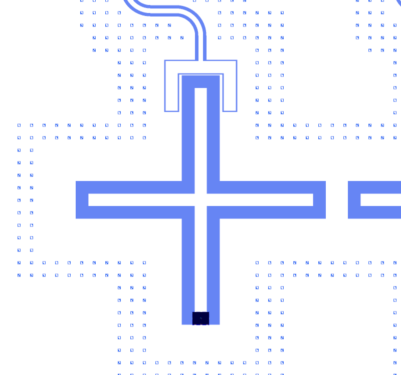
Tutorial 4, Q1 before the user revision (section 12, “before”).
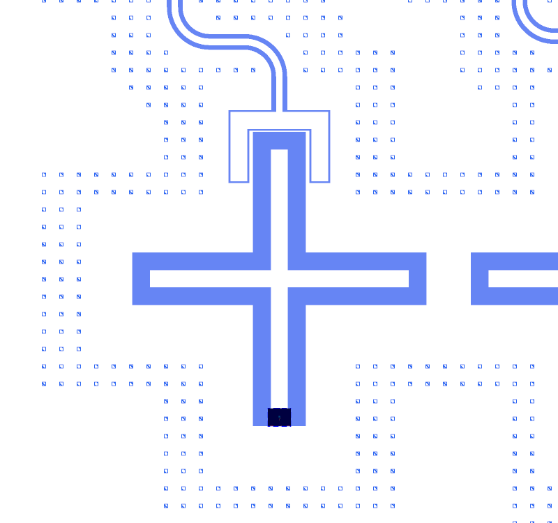
The same qubit after the user revision (“I want f_q1 = X”, section 10), as drawn in section 12 of tutorial 4.
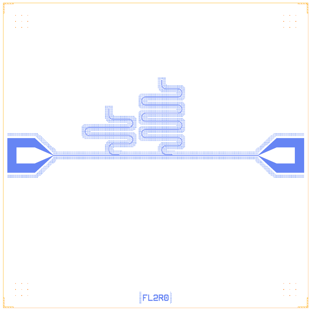
examples/fem_loop, revision 0 (2026-11-04, six real FEM jobs): the feedline and meandered readouts.
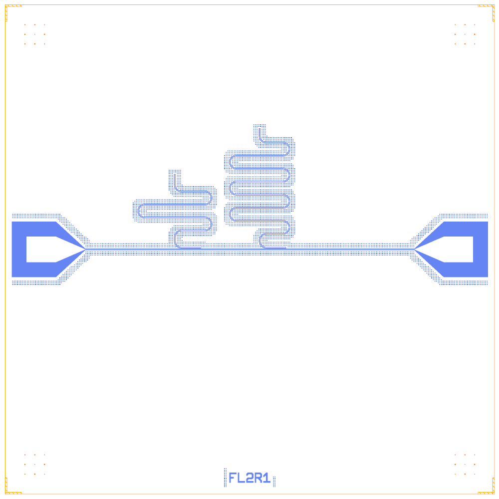
Revision 1: the meanders changed length and the FEM values moved with the geometry.
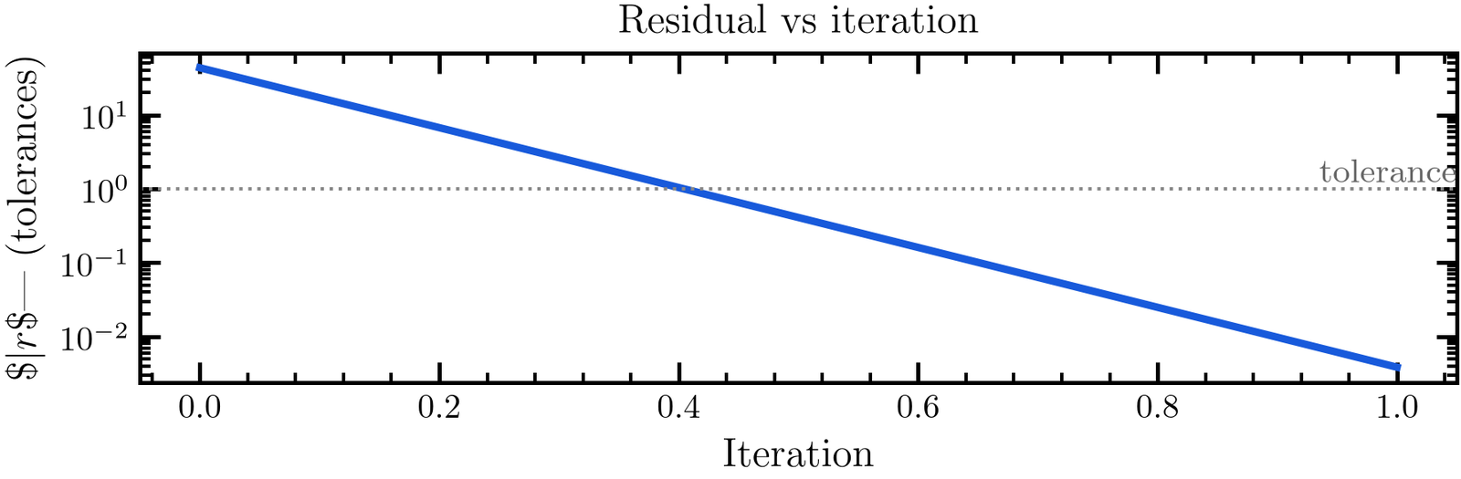
Residual against tolerance by iteration in the emulated loop. The dashboard’s History tab shows the same plot for a tracked run (dashboard).
A real FEM loop: tutorial 4
Tutorial 4 closes the loop with real FEM runs (2026-11-13, fast settings). Rev 0 FEM gave f_q1 5.011 and f_q2 5.294 GHz (targets 5.35 and 5.65). The correction FEM minus LOM gave a new LOM target; rev 1 FEM gave:
quantity |
target |
FEM rev 0 |
predicted rev 1 |
FEM rev 1 |
|---|---|---|---|---|
|
5.35 |
5.0108 |
5.3473 |
5.3613 |
|
5.65 |
5.2935 |
5.6466 |
5.6599 |
|
7 |
6.8702 |
6.9998 |
6.9831 |
|
7.3 |
7.1661 |
7.2998 |
7.3096 |
|
10 |
9.1923 |
10.5785 |
10.6894 |
The notebook ends with “rev 1 on target (FEM): False”: frequencies moved to within about 0.2 % of target but the tolerances (0.02 GHz for qubits, 0.01 GHz for readouts) are tighter. This is not a converged loop.
What is missing
FEM-sweep surrogates (Latin hypercube, single-element Palace or Elmer runs, RBF or GP), a Palace verify level, an HFSS sign-off level with a bias record in the PDK, and SQcircuit gradient levels are not built.
The loop was demonstrated for real once (tutorial 4). Other loops are emulated for at most 5 iterations (
test_codesign_track.py).test_propose_all.py: tolerances met rose from 9 to 78 to 81 of 84 targets.