Tutorial: draw Q1 + R1 in KLayout with the Quantcore plugin
You build examples/q1_r1_feedline.json by hand: one Xmon qubit (Q1) with a flux line, a λ/4 readout resonator (R1)
hanging off a feedline (FL), and three bond pads. Then you run the loop without simulating: Check → LOM → design.py →
Fab. It takes about 15 minutes. Nothing here edits JSON by hand.
The finished design:
Name |
What |
Where / values |
|---|---|---|
PAD_W, PAD_E |
|
(1125, 3750) rot 270 · (6375, 3750) rot 90 |
PAD_F |
|
(2964.5, 750) rot 0; a 4, b 6, pad_width 300, pad_height 300, pad_gap 150, taper_length 300 |
Q1 |
|
(2975, 2200); cross_length 300, arm_width 25, gap 25, claws |
FL |
route, cpw |
PAD_W.a → PAD_E.a |
R1 |
route, meander hanger |
Q1.claw_n → on FL at x ≈ 3125; length 4200 µm, coupler 300 µm, side right, ground strip 6 µm; targets f 7.2 GHz, g 90 MHz |
FLUX |
route, cpw |
PAD_F.a → node (2964.5, 1967) → Q1.flux; a 4, b 6; taper at the node to a 1, b 7.5 |
Before you start
Restart KLayout after the plugin code changes (a
git pullor an update). KLayout keeps the modules it loaded at start, so a half-updated plugin can show anImportErrorbox when the panel opens.The three toolbar modes: Move/Snap (place, move, double-click to edit), Connect (draw routes), Route handles (edit route nodes). KLayout’s own Select tool also works on components.
Undo / redo any design edit: Ctrl+Shift+Z / Ctrl+Shift+Y. Every step below is one undo step.
Clicks don’t need to be exact: each component’s dialog has exact x / y fields, and each route node has a node dialog. Zoom in when two ports are close; the capture radius is 12 pixels, so a click near a port takes the port.
1. New design
Quantcore ▸ Design ▸ New design… and save as, for example,
examples/hand_q1r1.json.The New design dialog asks for Die width µm and Die height µm. Leave Square die ticked and the width at 7500. (Untick it for a non-square die.)
The empty die builds and opens: frame, label, and the cheese band along the edge.
Optional: Design ▸ Chip settings… sets the label on the die to
Q1R1. Leave the KQC grid unticked.The same dialog sets the design’s substrate: thickness µm, εr (dk), loss tangent tan δ. The PDK’s sapphire values are preset (650 µm, 10.25, 1e-6). A changed value is stored in design.json as
"pdk": "quantcore_nb_sapphire_v1+substrate(eps_r=11.45)". The length estimates in the route dialogs, the LOM and the simulation exports all use it. For example, εr 11.45 moves Q1 + R1’s LOM resonator from 6.65 to 6.33 GHz.
2. Place the pads
Ctrl+Shift+P opens the Quantcore panel. In the Components tab, choose the library
quantcore.West pad. Double-click
BondPad. The outline follows the mouse. Press ] until the port arrow points east (into the chip), then click near (1125, 3750).East pad. Double-click
BondPadagain, press [ until the arrow points west, and click near (6375, 3750).Flux pad. Click
BondPadonce to show its parameters in the table, then seta4,b6,pad_width300,pad_height300,pad_gap150 andtaper_length300. Double-clickBondPad, check that the arrow points up (north), and click near (2964.5, 750).Exact positions. Switch to Move/Snap and double-click each pad. Type the x µm, y µm and rotation from the table above and press OK.
Names. The plugin names parts
BP1,BP2,BP3. Select one and use Edit ▸ Rename selected component… to rename themPAD_W,PAD_E,PAD_F. Optional, but the rest of this guide uses these names.
Snapping while you drag or place. A component that follows the mouse (picked up in Move/Snap, or armed with a
double-click in the panel or Duplicate) snaps by its ports. When one of its ports comes within the capture radius
of a compatible port (same CPW a / b) the component turns to face it and sits on it: the green square marks the
target and the label says which ports and how far it turned. Without a snap the rotation stays on the 90° steps of
[ / ]. The turn can be any angle, so the angled ports work: a Quantum Metal StarQubit has pins 72° apart,
a ConcentricTransmon couplers 60° apart.
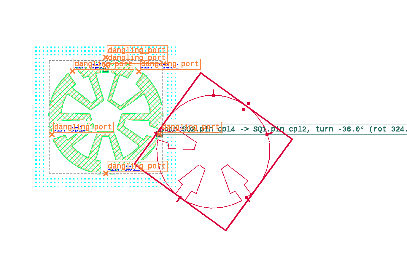
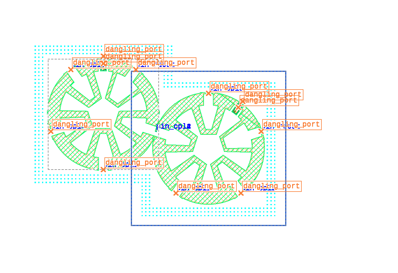
Click, and the placement is stored as place.snap (the port and its target); the build solves the same rotation, so
the built component lies exactly where the preview was:
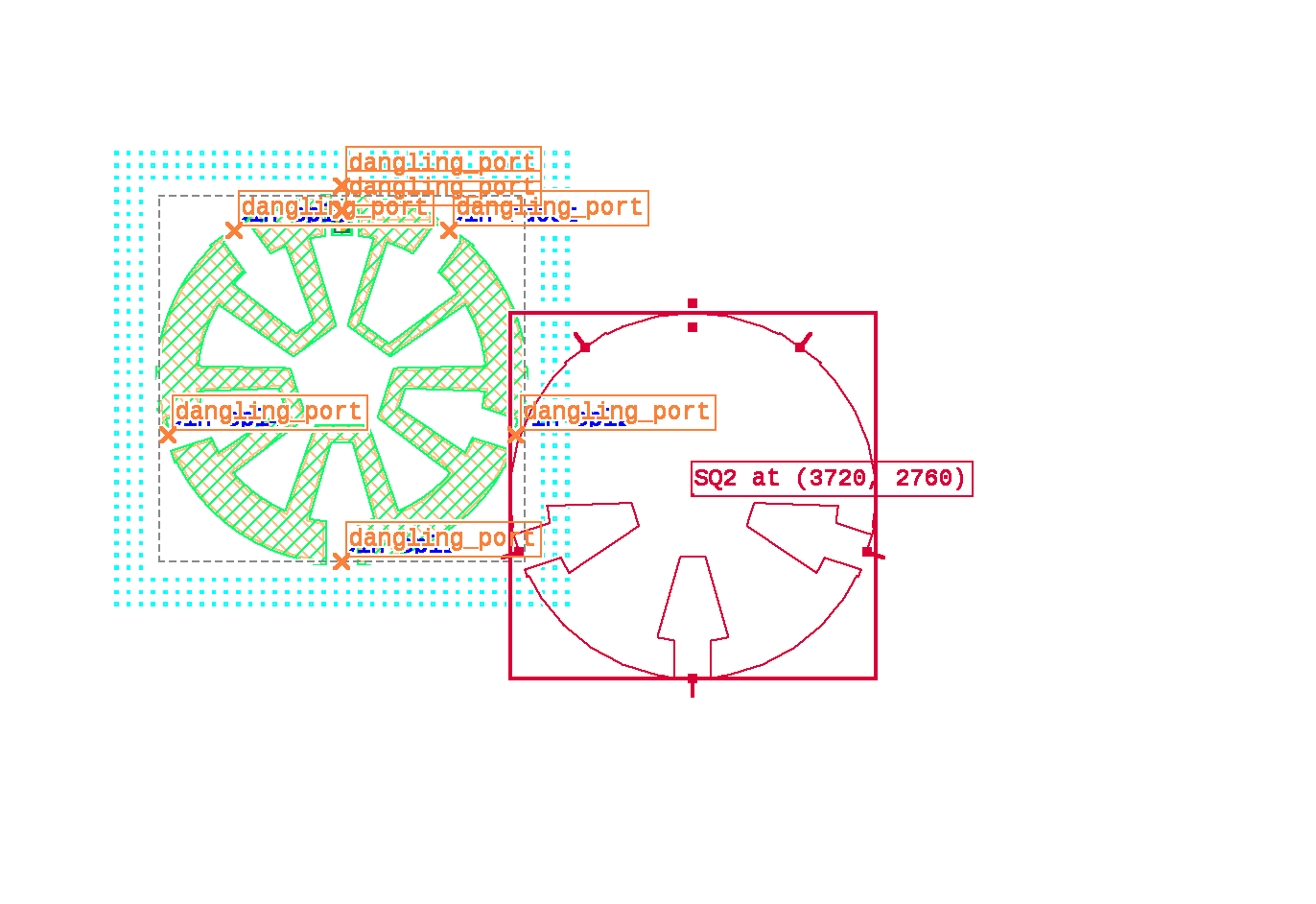
Hold Ctrl while moving for no rotation snap: only ports that already face each other (within 2.5°) snap, and the rotation stays what you set with [ / ].
3. Place the qubit
Click
Xmonin the list. In the table setjunction_typeTrilayer Squidandflux_porttrue.clawsis["n"]andcross_length300 already.Double-click
Xmonand click near (2975, 2200).In Move/Snap, double-click it and set x 2975, y 2200. Set the targets: f_q 5.1 GHz, α −220 MHz. Press OK.
Rename it
Q1.Junction. The same dialog has a section “Junction (simulation and LOM only, not drawn, not in the fab mask)”. These are simulation values: the junction you draw (
junction_type) is for fab only, and the value the LOM and the eigenmode run use is fixed per component in design.json. Enter L_J 12 nH and C_J 2 fF. L_J, I_c and R_n are one value (L_J = Φ0/2πI_c, I_c·R_n = πΔ/2e with the PDK’s Nb gap Δ = 1.4 meV), so you can type any one of them and the other two follow: L_J 12 nH is I_c 27.4 nA, R_n 80.2 kΩ. design.json keeps L_J and C_J (junction.Lj_nH,junction.Cj_fF). A SQUID (thisTrilayer Squid) also has flux Φ/Φ0 and asymmetry d (empty = 0, the sweet spot; L_J is then its value at zero flux), and the read-only rows show L at this bias (L_J / √(cos² πΦ + d² sin² πΦ), live while you type), the source of the value and the drawn junction (PDK) the cell draws, so you can see when a fixed simulation value no longer matches the drawing. Φ = ½ with d = 0 has no finite L and is shown in red. Without L_J the LOM has no qubit, and an eigenmode simulation cannot model the junction.A qubit you place gets its junction at placement: a drawn trilayer junction gives its PDK value (a KQC qubit left at its default junction is drawn as the PDK Quantcore Squid), a chosen KQC type (Manhattan, …) the PDK nominal SQUID (L_J 6.73 nH, C_J 15 fF), and the status bar says so (“Q1: junction L_J 6.73 nH (PDK nominal SQUID; simulation value, edit in the component dialog)”). Edit it here whenever you like.
Circuit rows. At the bottom, the component dialog lists the component’s circuit as the last build’s LOM sees it (read-only): C_Q1 to ground, the claw coupling, J_Q1 with L_J / C_J, each with where the value comes from. A route’s dialog lists its line (length → bare frequency, Z0) and its hanger coupling (κ). Run LOM and Simulate refine these values.
4. Feedline
Switch to Connect. Click
PAD_W.a(the port arrow turns red under the cursor), then clickPAD_E.a.In the route dialog, set the name
FLand the typecpw, and press OK. The feedline builds straight across.
5. Readout resonator (the hanger)
There is no coupler component: the hanger is the coupler. Any qubit port works the same way (Xmon claw,
TwoPadTransmon left/right, Flipmon coupler, a Metal qubit’s pin). A port that faces the line gives the cleanest
route. A port that faces sideways also works: the router goes around with extra corners. A Gatemon’s readout is
the island edge and no CPW end. Route from it and the dialog presets the PDK line width (10 / 6 µm), or snap a
GatemonCoupler to it and route from the coupler.
Still in Connect, click Q1’s claw port
Q1.claw_n(at the top of the qubit).Move up to the feedline. The preview shows a square corner, and the label reads “hang from FL here”. Click on the feedline at about x 3125, just above and right of the claw.
The hanger dialog opens:
leave Merge into FL (T-junction) unticked (that is section 11);
Name
R1, typemeander;Meander length µm 4200. The dialog shows the bare λ/4 frequency on the design’s εr as you type. A claw or a coupler pulls it lower: 7.5 GHz bare, 6.65 GHz in Q1 + R1’s LOM;
Coupler length 300, Side right, Coupler end short (λ/4), Ground strip 6;
Line width a and Line gap b: leave them empty. They are R1’s own CPW (centre line and the gap on both sides), over its whole length; empty takes the claw port’s;
the two Coupler: … facing … rows: leave them empty for this design (both 6 µm). Each narrows one gap along the coupler only, R1’s gap on the feedline’s side and FL’s gap on R1’s side. See step 7;
Direction: leave the preset.
Press OK. The meander fills the longest free straight between the claw and the coupler.
Targets. Switch to Route handles and double-click R1 on a straight, away from its nodes. The route dialog opens with a targets section: set f 7.2 GHz and g 90 MHz.
Meander on straight chooses which straight of the route holds the meander. The straights count from the route’s start (segment 1 leaves the claw), and the port stubs and the coupler are left out. Each entry shows the straight’s length, and the one you double-clicked is marked. automatic is the longest free straight. Leave it on automatic unless you want the meander elsewhere (Ctrl+Shift+M in Route handles does the same for the straight under the cursor).
Change it later. The same dialog holds everything the hanger was drawn with:
Coupler length, Side, Coupler end, Ground strip, Open gap, Direction;
the meander’s length, Meander turns (empty = automatic) and Meander first turn (flips the meander to the other side of its straight);
Merge into FL.
The dialog opens three ways: double-click the route in Route handles, double-click it in Move/Snap (a route is not a component, so this opens the route dialog), or select it with KLayout’s Select tool and press Ctrl+Shift+Q (Edit selected). KLayout’s own Object properties ▸ User properties only shows the instance’s
id. It is KLayout’s dialog and does not write design.json.A closer, stronger coupler: narrower facing gaps. Along the coupler, the resonator’s gap on the feedline’s side and the feedline’s gap on the resonator’s side can be narrower than the CPW’s 6 µm. Set Coupler: this route’s gap facing the line and Coupler: FL’s gap facing this route, for example 3 µm each, and the Ground strip, for example 4 µm. The two centre lines come closer by what the gaps save (28 µm apart becomes 20 µm). The outer gaps keep 6 µm. The build draws the extra ground over the coupler length, so it is in the fab mask and in the simulations. The LOM’s κ estimate follows: Q1 + R1 goes from 0.16 to 0.79 MHz. Empty fields mean the normal gap. A gap narrowed by more than the facing gap plus the ground strip is refused, because the etch would cut into the other line.
6. Flux line, with a taper
In Connect, click
PAD_F.a.Hold Shift and click at about (2964.5, 1967), straight above the pad. Shift snaps the segment to 0°, 45° or 90°, so this one is exactly vertical. (Hold Ctrl instead to place a node at any angle: the segment to it is one oblique straight.)
Click
Q1.flux(the small port under the qubit; zoom in if the claw or the cross takes the click).In the route dialog, set the name
FLUX, typecpw, Line width a 4 and Line gap b 6. Press OK.The taper. Switch to Route handles and double-click the node at (2964.5, 1967). The node dialog opens (the same as Edit ▸ Route node properties…, Ctrl+Shift+N, for a selected node). Set x 2964.5 and y 1967 exactly, Taper: line width a 1 and Taper: line gap b 7.5, and press OK. From that node to the qubit the line narrows to 1 / 7.5 µm.
7. Shape the routes (optional)
In Route handles:
click a node to pick it up and click again to drop it (any angle on the grid; Shift aligns it with its neighbours at 0° / 45° / 90°, or onto an angled port’s axis; a node off the axes makes an oblique straight, which a meander can use too); double-click a node for its dialog (exact x / y, corner radius, airbridge, taper);
filled squares are nodes: every corner of a route, including the corners the router drew by itself (a hanger meander from Connect without clicks). Move one, double-click it for its dialog, right-click it, or select it and press Ctrl+Shift+X (or Delete) to delete it. The first edit of a router corner writes all of that route’s corners to design.json, so the route keeps the shape the red preview shows;
hollow squares are not nodes: each sits in the middle of a straight and adds a node there (pick it up, drop it where the new corner goes). Nothing to delete. Port stubs and the hanger coupler have neither: the router keeps them straight;
lengthen a meander’s straight by moving its nodes apart, or move the meander to another straight (Ctrl+Shift+M, or Meander on segment in the dialog). When the meander no longer fits on its straight after an edit, the build puts it on the next longest free straight. If none can take it, the status bar says to lengthen one. A node moved off the coupler’s approach gets the corner that enters the coupler straight;
a selected corner shows a green curvature handle: drag it to set that corner’s bend radius by eye. For an exact value, use the node dialog (Corner radius µm). Leave it empty to use the route’s radius;
point at a straight and press Ctrl+Shift+M to move R1’s meander there;
double-click a route to reopen its dialog (length, radius, a / b, targets, and for a route that ends on a line: merge or hang, section 11);
a route that fails (for example two nodes 14 µm apart, too close for the bends) does not block the design: the rest builds, the status bar says
Route FLUX failed: ..., and the route is drawn in red with its handles. Move or delete its nodes, double-click it for the reason and Delete this route, or press Undo. Once it builds again the red goes away. The LOM keeps using its last good route (with a warning) meanwhile, and the fab export refuses until it is fixed.
KLayout’s Select tool draws a route’s selection box around the route itself (a meander’s box includes its meander).
8. Check
Click Check in the Flow strip at the top of the panel, or press Ctrl+Shift+D. The DRC tab lists:
errors (open ports, overlaps, crossings, opens or shorts): there should be none;
design warnings (PDK margins, the 100 µm pad-edge rule). At the positions above they should be clean. If a pad warns, Check and LOM ▸ Fix pad edge warnings moves it onto the edge rule.
Click a line in the DRC tab to zoom to it.
9. LOM
Click LOM in the Flow strip (or Ctrl+Shift+O). The LOM tab shows:
a progress bar with the stage (export, read, QuCat + QuTiP, write, draw) and the elapsed time;
a log of what
qccprints while it runs;when it ends (a few seconds for Q1 + R1): parameters against your targets (green = within tolerance, red = off), the modes, the netlist values, the circuit picture (click Open the circuit picture full size), and the connectivity of the layout.
Press Stop (beside Run LOM) to cancel a run: only the LOM process the panel started is killed, its partial output is discarded and the tab shows what it showed before the run.
A LOM run stops by itself when it fails, with the error in the log and a hint. It also stops after the time limit
(Quantcore ▸ Settings… ▸ Run LOM time limit, default 30 minutes), so a QuCat solve that never ends can’t hang
the panel. Q1 + R1 should land near f_q 5.1 GHz and f_r 7.2 GHz. To compare, run
qcc circuit simulate examples/q1_r1_feedline.json in a terminal.
10. Save as Python and export for fab
Design ▸ Save as Python script (design.py)… writes a Designer script that rebuilds this exact design (the design hash is checked). Continue the chip in code from there.
Fab ▸ Export for fab (mask, netlist, design.py, PNG)… writes
<name>_fab.oas(PDK layers, cheese, frame),circuit.json,design.pyand a PNG into a folder you choose. It warns first if Check found errors.
Results / Propose / Apply come after a simulation (section 14).
11. More ways to end a route on a line
A resonator that is not attached to a qubit
A route can start on empty canvas: that start is a free end, open or shorted, so you need no open/short component.
In Connect, click empty canvas where the resonator should start. A hollow red square marks the free end.
Click nodes as usual (Shift for straight 0 / 45 / 90° segments), then click on the feedline.
In the hanger dialog, Free end (start) chooses
open(with the Open gap µm) orshort. Typemeanderand a length make it a λ/4 (short) or λ/2 (open) resonator hanging off the line.
A route can also end free: click the last node again. The route dialog then asks for the end’s open/short.
CpweOpenEnd (Quantcore) and metal:OpenToGround / metal:ShortToGround are termination components, if you want a
named part at the end. A free end does the same job without one.
Merge into the line (T-junction) instead of hanging beside it
A hanger couples beside the line. To join the line itself, for example a finger capacitor between the feedline and a resonator, merge into the line:
Place the capacitor (for example
CpweFingerCapacitor, rotated so a port faces the feedline).In Connect, click the capacitor’s port, then press Ctrl+Shift+J (Quantcore ▸ Edit ▸ Connect on a line: hang / merge). The label changes from “hang from FL here” to “merge into FL here (T-junction)”. Press it again to switch back. The default is hang. Plain T would be KLayout’s own Selection ▸ Tap.
Click on the feedline. The dialog opens with Merge into FL (T-junction) ticked and the type
cpw. Ticking or unticking the box in the dialog decides for this route, whatever T was set to.OK splits FL into
FLandFL_1, joined by a T (T1, a KQCWaveguideCoplanarSplitterdrawn in the line’s width), and the route ends on the T’s stemT1.c. A hanger on the second half moves toFL_1. The T needs 11 µm + 2 bend radii of straight line on both sides; closer to a corner, the status bar says so.
To change it later, double-click the route in Route handles. A route that ends on a line shows the same checkbox. Untick it and the T goes away: the two halves become one line again, and the route ends in a 300 µm hanger coupler there. Tick it again to merge. In the LOM the T is one conductor, so the capacitor sits galvanically on the line.
12. Component classes
Every component has a class: qubit, junction, coupler, capacitor, resonator, launcher, termination,
waveguide, airbridge, marker, test_structure, flip_chip, shape, other. Use the second drop-down in the
Components tab to filter by class. Hover over a component to see its class and description. qcc components lists
them by class from the command line.
What the class gives a component:
qubit: the edit dialog offers qubit targets (f_q, α). Junction values (Lj, Cj) feed the LOM’s junction. Every qubit cell gets them, from any library (Xmon, TwoPadTransmon, KQC
DoublePads,Swissmon, MetalTransmonPocket, …).resonator: resonator targets (f, κ). A route gets resonator targets whatever its type.
launcher: the pad-edge rule (100 µm from the die edge) and the device-ID placement.
junction: valid as any qubit’s
junction_type, and never offered qubit targets.
Each component still has its own parameters (the table) and its own LOM model. Classes share behaviour through
Python inheritance. A cell that subclasses a KQC Qubit gets the junction parameters (junction_type, …), and a
LOM model registered for a class name also covers its subclasses.
13. Make your own component
A component is a KQCircuits Element class in one Python file. The worked example is
examples/custom_component/pad_gap_capacitor.py: two pads
facing across a gap in a CPW line.
Write the class. Subclass
kqcircuits.elements.element.Elementand add:qcc_category = "capacitor"(the class, section 12);one
Param(...)per parameter, with a description, default and unit. The panel’s table shows these;build(self), which draws the etched region (negative mask) onself.get_layer("base_metal_gap_wo_grid"). Callself.add_protection(...)where no cheese may go;self.add_port("a", pya.DPoint(x, y), pya.DVector(dx, dy))for each port, with the direction pointing out of the component. A route leaves and arrives along that direction. Without a direction the port is a point, like a squid’s ends.
Put it in the library. Copy the file into
src/quantcore_circuits/layouts/others/(orqubits/,junctions/); file names starting with_are skipped. A separate package can instead declare aquantcore_circuits.cellsentry point (seesrc/quantcore_circuits/plugins.py).Check it in a terminal:
qcc components PadGapCapacitorlists its ports;qcc components PadGapCapacitor --schemalists its parameters.
Restart KLayout. The component is now in the Components tab (library
quantcore, classcapacitor). Place it, edit its parameters, and Connect to its ports like any other.LOM model (optional). Decorate a function with
@register_lom("PadGapCapacitor")that returns aFragment:nodes: the component’s conductors;port_nodes: which conductor each port touches;elements: C / L / JJ between conductors or to"gnd", with values fromquantcore_circuits.lom.estimates. The example keeps its model in the same file. Without a model, Run LOM notes that the component has none.
The example lists with class capacitor, builds in a design (pad → capacitor → λ/4 meander), passes DRC, and gives
an LOM of 7.37 GHz with κ 6.6 MHz from its own model.
What to look for
Report any of these:
anything that needs a second try: a click that took the wrong port, a preview that differs from what is placed, a dialog that loses a value;
a Script Error box (there should be none: errors go to the status bar and
%TEMP%\qcc_kplugin.log);a panel that grows and squeezes the layout view;
values that differ from the table above after a rebuild.
Known gaps:
simulation groups are made by Simulate, not drawn;
segments at angles other than 0 / 45 / 90° need an extra corner and the node dialog;
a route that fails to build has no handles until it builds;
a merge T sits on a straight part of the line, not on a corner.
14. Simulate: Q3D for qubits, eigenmode for resonators and lines
Select what to simulate with KLayout’s Select tool, then press Simulate in the Flow strip. The dialog shows what it will render and lets you choose the analysis:
Q3D capacitance: for qubits (alone, or with couplers and capacitors). The qubit’s islands and couplers become nets, and the resonator is cut to a short stub port, so only the qubit is drawn. The result is the C matrix the LOM uses (C_Σ, the claw coupling). This is preselected when you select only qubits.
HFSS eigenmode: for a resonator, a feedline, pads, or a qubit with its readout. Everything selected is drawn, plus the routes that join two selected parts and the pads at the ends of a selected line. The junction is a lumped L‖C port with your L_J / C_J, and the pads and any line cut by the box end in 50 Ω ports. The result is the modes’ f and Q (κ, χ). This is preselected when the selection has a line, a resonator or a pad. A qubit without L_J is named in red, with where to set it, and the run and export buttons stay disabled until you set it (L_J, I_c or R_n in the component dialog’s junction section). With nothing selected the default subset is checked the same way.
Nothing selected: the default subset (the first qubit with its readout) or the whole chip.
Open simulation layout… (a button of this dialog and Simulate ▸ Open simulation layout…) exports the job geometry of the selection, the default subset or a saved sim group, with no AEDT, and opens the GDS that AEDT imports in a new layout tab: the cut-out metal and gaps on readable layers, the junction sheet and the port polygons as extra layers. It is the quick way to see what HFSS gets before you solve. Your design and its build are not touched; closing the tab may ask to save (answer No). For eigenmode it checks the junctions first, like the dialog: a qubit of your own without an L_J opens a window that names it, with a button for the Q3D layout instead.
What will be simulated is drawn in the layout while the dialog is open (and follows the analysis you pick): a
purple box (the box of the export, with its group, analysis and size), the selected components in green frames, the
routes that stay in the simulation as green lines (a grey one only passes through the box, like a feedline the box
cuts), other components that reach into the box dashed grey, and the ports: the junction in red, 50 Ω terminations
(the pads, or a line cut by the box) in blue, a cut resonator’s stub port in orange with the stub drawn from the
component’s port. The drawing comes from qcc sim preview (the library’s own build_simulation, so the box, ports
and routes are exactly those of the job folder that Export the job only writes) and exists only in KLayout: it is
never on a fab layer and is not in any export. It disappears when the dialog closes.
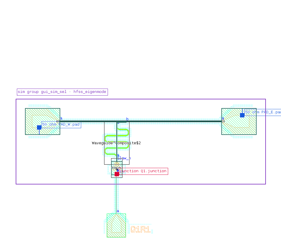
Saved groups. The panel’s Sim groups tab lists the sim_groups of design.json (the Simulate dialog writes
gui_sim… groups there). Click one to draw it the same way, pick the analysis it is drawn for, and press Hide to
remove it. It stays until hidden, is drawn again after each rebuild, and is previewed again when the design changes.
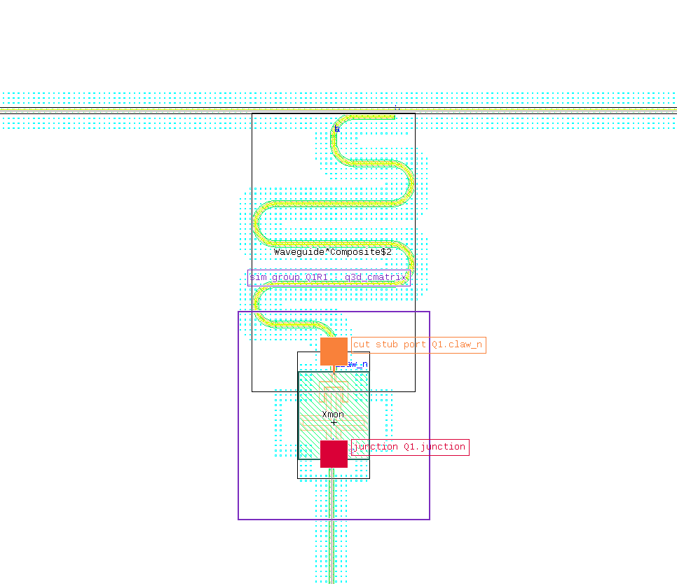
To go qubit by qubit: select Q1 alone → Q3D (its capacitances), then Q1 + R1 + FL (+ pads) → eigenmode (the readout and the qubit together). The two runs fill different parts of the LOM.
Solver settings: below the analysis, the dialog shows the settings of the run, filled with the fast values (minutes; the values move with the design but are not converged):
Q3D: convergence ΔC per pass 2 %, at most 8 adaptive passes, 1 converged pass in a row;
eigenmode: 2 modes above 3 GHz, Δf per pass 1 %, at most 3 passes, 1 converged pass, 30 % mesh refinement per pass, and mesh seeds of 40 µm on the CPW gaps and 10 µm on the junction islands (empty = no seed).
Change any of them before you press Simulate (for example 12 passes and 0.5 % for a finer Q3D). Your values are kept
for the next run; Reset to the fast values puts the fast ones back. Full-wave driven (S-parameter) runs are left to
scripts (qcc sim … -a hfss_driven).
Convergence, and a finer run: after each Simulate run Quantcore reads AEDT’s convergence table by itself and
stores it in build/<design>/convergence.json. The next Simulate dialog shows it, for example “Last Q3D run:
converged in 4 passes” or “NOT converged after 3 passes (last Δ 2.1 vs target 1.0): raise the maximum passes in AEDT,
solve there and import the job folder”. For a converged result:
open the job’s
<sim>_project.aedtin AEDT (the job folder is underbuild/jobs/), change the setup (passes, convergence, mesh) and solve;in that AEDT, run the job’s
scripts/qcc_collect.py(Tools ▸ Run Script…, no arguments). It exports what you solved, results and convergence table, into the job folder, without solving again or saving. If the link to that AEDT is broken, close the project there and runqcc hfss collect <job folder>instead (a new non-graphical AEDT does the same);Simulate ▸ Import results… and pick the job folder. A folder whose AEDT outputs are newer than its results is read again, and its convergence table with it; the status bar and the Results tab show the new values.
Closing KLayout while it runs: Simulate runs detached, so quitting KLayout does not end it. Open the design
again later (or restart KLayout with it): a run that finished meanwhile is imported and shown in the Results tab, and
one still going is reported and imported when it ends. Its output is in build/<design>.flow/sim_run.log, and what the
solve returned is saved as build/<design>/<design>_<group>_results.json. Simulate ▸ Import results… reads such
a file (pick “A results.json file”) or a solved job folder.
Export the job only (a button of the Simulate dialog) writes the job folder (geometry, AEDT scripts, README) with the same analysis and settings, to solve by hand or on another machine.
The same from a terminal (qcc): in the conda environment, from the design’s folder:
What |
Command |
|---|---|
what a selection would render: box, components, ports as JSON (nothing is written) |
|
export the job of a selection (no solve) |
|
eigenmode of qubit + readout + feedline (the pads come with the line) |
|
your own settings on top of the defaults |
add |
check an exported job before AEDT (what Simulate does) |
|
export, solve in a new non-graphical AEDT and analyse (what Simulate does) |
|
solve an exported job |
|
re-export what you solved in AEDT (no re-solve; close the project there first) |
|
read a solved job folder (or a |
|
the results format |
|
A Q3D run needs no junction values; an eigenmode run needs L_J on every qubit in the box. Never point qcc at the
AEDT you have open: qcc sim auto and qcc hfss collect start their own.
Propose the next revision
Set targets first (in the qubit’s and the resonator’s edit dialog, or targets in design.json: f_q and α for Q1, f_r
and g for R1). Then
Results ▸ Propose next revision… (qcc results propose design.json -o proposal.json in a terminal) turns the
values against the targets into new knob values. It uses the last simulation’s results, or the layout’s own LOM
estimates when there is no simulation yet, and it tunes every qubit with a readout resonator, whatever its class
(Xmon, Swissmon, DoublePads, TwoPadTransmon, Flipmon, Gatemon, the Metal pockets and crosses, …) and whether the readout
is λ/4 or λ/2. For each qubit–readout pair it moves:
L_J (
Q1.junction.Lj_nH) for f_q,the island knob for α (here the Xmon’s
cross_length; a TransmonPocket’spad_width, …),the coupler knob for g (here
claw_length; a pocket’sconnection_pads.<pad>.pad_width, …),the resonator length (
R1.length) for f_r.
A knob whose target is not set stays where it is. The window lists each knob’s value now and proposed, the waypoints
that follow a moved port (also: …, e.g. the flux line’s taper when the cross grows), the predicted distance from the
targets, and under Not tuned what it could not change and why: a junction drawn without an L_J in design.json, a
readout drawn as a plain route without a length, a qubit with no readout. On examples/q1_r1_feedline.json (targets
f_q 5.1 GHz, α −220 MHz, f_r 7.2 GHz, g 90 MHz) it proposes cross 300 → 415.8 µm, claw 100 → 187.9 µm, L_J 12 →
9.28 nH and R1 4200 → 3555.6 µm.
Apply and rebuild writes the values to design.json (one undo step) and rebuilds; then simulate (or Run LOM) again
to check: the prediction comes from a surrogate of the LOM, and a second Propose closes what is left. A second Propose
without a change in between, or one right after Import results, reuses the analysis (build/<name>/ estimates_cache.json) and takes a few seconds. From a terminal: qcc results apply design.json proposal.json -o design_rev1.json (it refuses when the design changed since the proposal).